 . It is defined as the averaged flux of Γ through the infinitesimal
poloidal surface dS
. It is defined as the averaged flux of Γ through the infinitesimal
poloidal surface dS
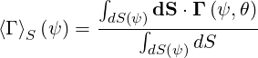
We consider the flux-surface averaging of a surface quantity, such as a flux of a current,
generally noted Γ . It is defined as the averaged flux of Γ through the infinitesimal
poloidal surface dS
 | (3.227) |
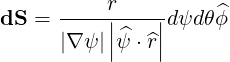
In the  system, the differential poloidal surface element is given by (A.201) as
introduced in Appendix A
system, the differential poloidal surface element is given by (A.201) as
introduced in Appendix A
 | (3.228) |
so that the infinitesimal poloidal surface element dSp is
is
 | (3.229) |
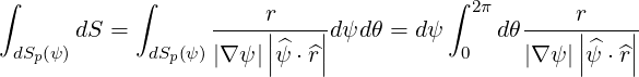
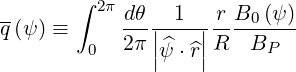
and the flux-surface averaged flux in the toroidal direction is
![( ) -1∫ 2π [ ]
⟨Γ ⟩ (ψ) = dSp- dθ----r|---|- ^ϕ⋅Γ (ψ,θ)
ϕ dψ 0 |∇ψ |||ψ^⋅^r||](NoticeDKE675x.png) | (3.230) |
with
 | = ∫
02πdθ | (3.231) |
= ∫
02πdθ   | (3.232) |
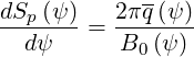
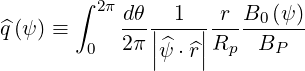
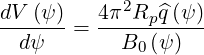
Defining the new pseudo saftey factor q as
 | (3.233) |
we get
 | (3.234) |
and
![∫ [ ]
⟨Γ ⟩ (ψ) = --1-- 2π dθ|--1-|r-B0-(ψ) ^ϕ⋅Γ (ψ,θ)
ϕ q(ψ ) 0 2π||^ψ ⋅^r||R BP](NoticeDKE683x.png) | (3.235) |
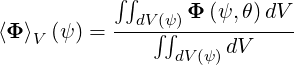
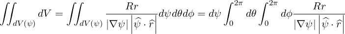
We consider the flux-surface averaging of a volume quantity, such as a power density, generally
noted Φ . It is defined as the average value of Φ within the infinitesimal volume
dV
. It is defined as the average value of Φ within the infinitesimal volume
dV 
 | (3.236) |
In the  system, the differential volume element is given by (A.202) as introduced in
Appendix A
system, the differential volume element is given by (A.202) as introduced in
Appendix A
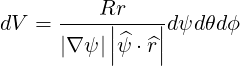 | (3.237) |
so that the infinitesimal volume element dV  of a flux-surface is
 | (3.238) |
and the flux-surface averaged quantity in the toroidal direction is
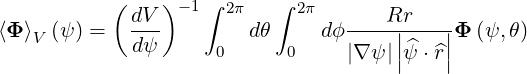 | (3.239) |
with
 | = ∫
02πdθ∫
02πdϕ | (3.240) |
= ∫
02πdθ∫
02πdϕ  | (3.241) |
Under the assumption of axisymmetry, we get
 | = 4π2 ∫
02π   | (3.242) |
=  ∫
02π ∫
02π    | (3.243) |
Defining the new pseudo saftey factor  as
as
 | (3.244) |
we get
 | (3.245) |
and finally
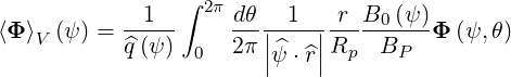 | (3.246) |
The electron density ne is given by the relation
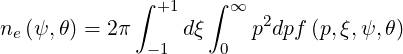 | (3.247) |
Using the general expression (3.246) of the flux-surface averaging of a volumic quantity
 V V  | =  ∫
02π ∫
02π    ne ne | ||
=  ∫
0∞p2dp∫
02π ∫
0∞p2dp∫
02π    ∫
-1+1dξf ∫
-1+1dξf | |||
=  ∫
0∞p2dp∫
02π ∫
0∞p2dp∫
02π    ∫
-1+1 ∫
-1+1![[ ]
1 ∑
--
2 σ=±1](NoticeDKE730x.png) T dξf T dξf | |||
| (3.248) |
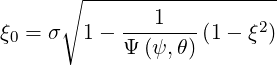
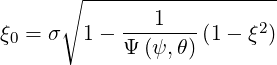
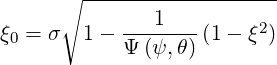
where the trapping condition evaluated at the location θ is given by
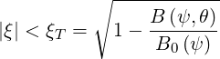 | (3.249) |
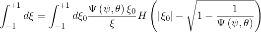
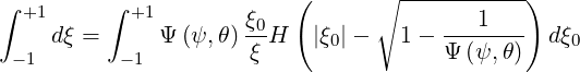
Using ξdξ = Ψξ0dξ0 with the condition (3.270) on ξ0
 | (3.250) |
one get
![∫ [ ] ∫ [ ] ( ∘ -----------)
+1 1-∑ +1 1- ∑ ξ0 ---1---
2 dξ = 2 Ψ (ψ,θ) ξ H |ξ0|- 1 - Ψ (ψ,θ) dξ0
-1 σ= ±1 T -1 σ=±1 T](NoticeDKE734x.png) | (3.251) |
where H is the usual Heaviside function which is defined as H = 1 for x > 0, and H
 = 0
elsewhere.
= 0
elsewhere.
Note that the condition (3.250) is equivalent to
 | (3.252) |
so that, the integrals over θ and ξ0 may be permuted,
 V V  | =  ∫
0∞p2dp∫
-1+1dξ
0× ∫
0∞p2dp∫
-1+1dξ
0× | ||
![[ ]
1 ∑
--
2 σ=±1](NoticeDKE741x.png) T ∫
θminθmax T ∫
θminθmax
     f f | (3.253) |
where the bounce-averaging of the distribution appears naturally. Therefore, expression (3.371) can be rewriten in the simple form
 | (3.254) |
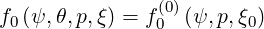
For the zero order distribution function, since f0 is constant along a field line,
 | (3.255) |
one obtains
 | (3.256) |
When we consider the first order distribution function, we have f1 =  + g, where g is
constant along a field line, and therefore its contribution
+ g, where g is
constant along a field line, and therefore its contribution  V 1
V 1 has the same
expression as for f0. However,
has the same
expression as for f0. However,  has an explicit dependence upon θ, which is given by
(3.206)
has an explicit dependence upon θ, which is given by
(3.206)
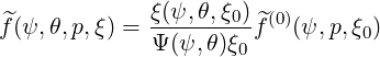 | (3.257) |
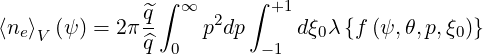
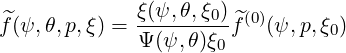
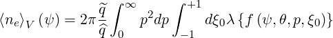
Therefore, the flux-surface averaged density contribution of  is
is
 V 1 V 1 | = 2π ∫
0∞p2dp∫
-1+1dξ
0λ ∫
0∞p2dp∫
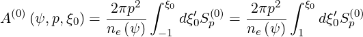
-1+1dξ
0λ  (0)(ψ,p,ξ
0) (0)(ψ,p,ξ
0) | (3.258) |
= 2π ∫
0∞p2dp∫
-1+1dξ
0λ1,-1,0 ∫
0∞p2dp∫
-1+1dξ
0λ1,-1,0 (0)(ψ,p,ξ0) (0)(ψ,p,ξ0) | (3.259) |
where
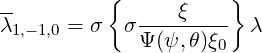 | (3.260) |
according to the notation in Sec. 2.2.1, since  (0) is antisymmetric in the trapped
region.
(0) is antisymmetric in the trapped
region.
Since  (0) and g have no definite symmetry properties, both can contribute to the density
and
(0) and g have no definite symmetry properties, both can contribute to the density
and
 | (3.261) |
The density of current carried by electrons is given by
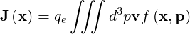 | (3.262) |
so that the parallel current density is
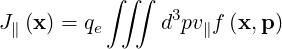 | (3.263) |
which becomes in  phase space
 | (3.264) |
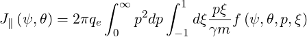
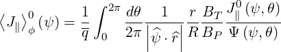
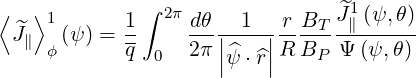
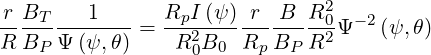
We are usually interested in the flux-surface averaged current density in the toroidal direction. It is generally given by (3.230)
 ϕ ϕ | =  ∫
02π ∫
02π    J∥ J∥ ![[ ]
^ϕ⋅^b](NoticeDKE780x.png) | ||
=  ∫
02π ∫
02π    J∥ J∥  | (3.265) |
and finally, using (2.23)
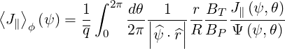 | (3.266) |
When we consider only the zero order distribution function, we have that f0 is constant along a field line, so that
 | (3.267) |
where
 | (3.268) |
Consequently, we find
J∥0 | = 2πq
e ∫
0∞p2dp∫
-11dξ f0 f0 | ||
= 2πqe ∫
0∞p2dp∫
-11dξ f0(0) f0(0) | |||
= 2πqe ∫
0∞p2dp∫
-11dξ
0Ψ × × | |||
H  f0(0) f0(0) | (3.269) |
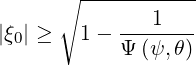
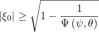
where the condition
 | (3.270) |
results from the equation (3.268) and means that only the particle who reach the position θ must be considered. Note that the integrand in the equation (3.269) is odd in ξ0 for trapped electrons, since f0(0) is symmetric in the trapped region. As a consequence, the contribution from trapped electrons vanishes, and (3.269) can be rewritten as
 | (3.271) |
Therefore, the flux-surface averaged current density
 | (3.272) |
becomes
 ϕ0 ϕ0 | =  ∫
0∞dp ∫
0∞dp  ∫
02π ∫
02π     × × | ||
∫
-11dξ
0Ψ H H ξ0f0(0) ξ0f0(0) | (3.273) |
The integrals over θ and ξ0 can be permuted
 ϕ0 ϕ0 | =  ∫
0∞dp ∫
0∞dp ∫
-11dξ
0H ∫
-11dξ
0H ξ0f0(0) ξ0f0(0) × × | ||
 ∫
02π ∫
02π    | (3.274) |
We recognize the expression of the safety factor (2.51) so that
 | (3.275) |
Case of circular concentric flux-surfaces In that case, we showed in (2.83) that the safety factor is
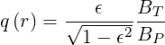 | (3.276) |
with ϵ = r∕Rp the inverse aspect ratio.
In addition, q becomes
q | = ∫
02π   | ||
= ∫
02π    | |||
= ϵ  | |||
=   | (3.277) |
since R = Rp + r cosθ, and B0∕B = R∕R0. We have then
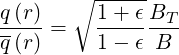 | (3.278) |
In the case when BT ≫ BP , we retrieve the bounce-averaged coefficient s* and in the large aspect ratio limit ϵ ≪ 1,
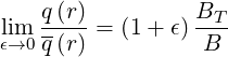 | (3.279) |
When we consider the first order distribution function, we have f1 =  + g, where g is constant
along a field line, and therefore its contribution has the same expression as for f0. However,
+ g, where g is constant
along a field line, and therefore its contribution has the same expression as for f0. However,  has an explicit dependence upon θ, which is given by (3.206)
 | (3.280) |
where
 | (3.281) |
Consequently, we find
 ∥1 ∥1 | = 2πq
e ∫
0∞p2dp∫
-11dξ   | ||
= 2πqe ∫
0∞p2dp∫
-11dξ   (0)(ψ,p,ξ
0) (0)(ψ,p,ξ
0) | |||
= 2πqe ∫
0∞p2dp∫
-11dξ
0 × × | |||
H   (0) (0) | (3.282) |
where again the condition
 | (3.283) |
results from the equation (3.268) and means that only the particle who reach the poloidal position θ must be considered.
Therefore, the flux-surface averaged current density contribution from 
 | (3.284) |
becomes
 ϕ1 ϕ1 | =  ∫
0∞dp ∫
0∞dp  ∫
02π ∫
02π     × × | ||
∫
-11dξ
0 H H ξ0 ξ0 (0) (0) | (3.285) |
Note that the condition (3.283) is equivalent to
 | (3.286) |
so that, permuting the integrals over θ and ξ0, we find
 ϕ1 ϕ1 | =  ∫
0∞dp ∫
0∞dp ∫
-11dξ
0ξ0 ∫
-11dξ
0ξ0 (0) (0) | ||
 ∫
θminθmax ∫
θminθmax
      | (3.287) |
We have then
 | (3.288) |
Then, noting the the integrand in (3.287) is independent of σ , so that the sum over σ for trapped particles can be added, we obtain
 ϕ1 ϕ1 | =  ∫
0∞dp ∫
0∞dp ∫
-11dξ
0ξ0 ∫
-11dξ
0ξ0 (0) (0)   × × | ||
![[ ]
1∑
2
σ](NoticeDKE901x.png) T ∫
θminθmax T ∫
θminθmax
     ![[ ]
R0-
R](NoticeDKE907x.png) 2Ψ-2 2Ψ-2 ![[ ]
ξ-
ξ0](NoticeDKE909x.png) 2 2 | (3.289) |
We recognize the expression of a bounce coefficients defined by the general relation (2.66) in Sec. 2.2.1, so that we get finally
 | (3.290) |
with
 | (3.291) |
Case of circular concentric flux-surfaces
In that case, we showed in (2.99) that  is
is
 | (3.292) |
with ϵ = r∕Rp the inverse aspect ratio.
In addition, q is
is
 | (3.293) |
and since
 | (3.294) |
we have then
 | (3.295) |
in the limit BP ≪ B.
Also, in this case,
 | (3.296) |
so that
 | (3.297) |
using notations used in previous publications. The exact expression of  * in terms of a series
expansion is given in relation (4.148).
* in terms of a series
expansion is given in relation (4.148).
The kinetic energy associated with a relativistic electron of momentum p is
 | (3.298) |
Then, the local energy density of electrons is
 | (3.299) |
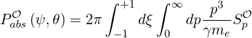
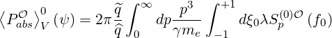
The density of power absorbed through the process  , Pabs
 , is
, is
 | (3.300) |
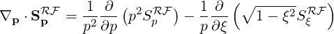
When the operator is described in conservative form, as the divergence of a flux
 | (3.301) |
then the power density becomes
![∫ ∞ ∫ +1 [ 1 ∂ ( ) 1 ∂ ( ∘ ------ )]
P Oabs = - 2πmec2 p2dp(γ - 1) dξ -2 --- p2SOp - ----- 1- ξ2SOξ
0 -1 p ∂p p ∂ξ](NoticeDKE925x.png) | (3.302) |
The integration of the Sξ term gives no contribution, since the particle energy is function of
p only
![∫ +1 ( ) [ ]
dξ ∂-- ∘1---ξ2SO = ∘1----ξ2SO +1 = 0
-1 ∂ξ ξ ξ - 1](NoticeDKE926x.png) | (3.303) |
and the equation (3.302) reduces to
 | (3.304) |
Integrating by parts, we get
![O 2∫ +1 ( [ 2 O]∞ ∫ ∞ dγ 2 O )
Pabs = - 2πmec dξ (γ - 1) p Sp 0 - dpp S p dp
-1 0](NoticeDKE928x.png) | (3.305) |
Assuming that limp→∞p2Sp = 0, and using
 | (3.306) |
the equation (3.305) reduces to
 | (3.307) |
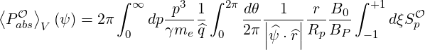
Starting from the general expression of the flux-surface averaging of a volume quantity (3.246),
the flux-surface averaged power density  V
V  is
is
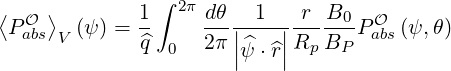 | (3.308) |
which becomes
 | (3.309) |
The sum over σ for trapped electrons can be added, using
∫
-11dξ![[ ]
1-∑
2
σ= ±1](NoticeDKE935x.png) T Sp T Sp | = ∫
-1-ξT
dξSp + ∫
ξT1dξS
p +  ∫
-ξTξT
dξ ∑
σ=±1Sp ∫
-ξTξT
dξ ∑
σ=±1Sp | ||
= ∫
-1-ξT
dξSp + ∫
ξT1dξS
p +  ∫
-ξTξT
dξ ∫
-ξTξT
dξ![[SO(ξ) + SO(- ξ)]
p p](NoticeDKE938x.png) | |||
| = ∫
-1-ξT
dξSp + ∫
ξT1dξS
p + ∫
-ξTξT
dξSp(ξ) | |||
| = ∫
-11dξS
p | (3.310) |
where the trapping condition evaluated at the poloidal location θ is
 | (3.311) |
Using ξdξ = Ψξ0dξ0 with the condition (3.270) on ξ0
 | (3.312) |
we get that
 | (3.313) |
Note that the condition (3.312) is equivalent to
 | (3.314) |
so that, permuting the integrals over θ and ξ0, we find
 V V  | = 2π ∫
0∞dp ∫
-1+1dξ
0 ∫
-1+1dξ
0 | (3.315) |
 ![[ ∑ ]
1-
2σ=±1](NoticeDKE947x.png) T ∫
θminθmax T ∫
θminθmax
     Sp Sp | (3.316) |
We see that the bounce-averaging of the fluxes appears naturally, so that we can rewrite
 | (3.317) |
Using the definition (3.167), we observe that the flux-surface averaged power density is calculated using the momentum flux component of the bounce-averaged kinetic equation:
 | (3.318) |
Case of circular concentric flux-surfaces
In that case, we showed in (3.292) that the coefficient  is
is
 | (3.319) |
with ϵ = r∕Rp.
In addition, 
 becomes
  | = ∫
02π   | ||
= ϵ ∫
02π ∫
02π  | |||
= ϵ ∫
02π ∫
02π  | |||
=   | (3.320) |
using the simple relation B∕B0 = R0∕R and R0 = Rp .
.
We have then
 | (3.321) |
The Fokker-Planck equation (3.107) solves for the zero-order distribution function f0.
The density of power transfered to f0 through the momentum-space mechanism is
then
 | (3.322) |
where Sp
 is given by (3.187)
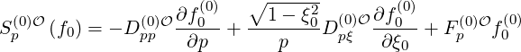 | (3.323) |
The momentum-space diffusion and convection elements Dpp(0), Dpξ(0) and Fp(0)
associated with a particular mechanism are calculated in chapter 4.
The Fokker-Planck equation (6.1) solves for the first-order distribution function f1 =  + g
(3.117). The densities of power transfered to
+ g
(3.117). The densities of power transfered to  and g through the momentum-space mechanism
are then respectively
and g through the momentum-space mechanism
are then respectively
 V 1 V 1 | = 2π ∫
0∞dp ∫
0∞dp ∫
-1+1dξ
0λ ∫
-1+1dξ
0λ p p  | (3.324) |
 V 1 V 1 | = 2π ∫
0∞dp ∫
0∞dp ∫
-1+1dξ
0λSp ∫
-1+1dξ
0λSp  | (3.325) |
where  p
p
 and Sp
 are given by (3.187) and (3.216)
 p(0) p(0) | = - pp(0) pp(0) + +   pξ(0) pξ(0) + +  p(0) p(0) (0) (0) | (3.326) |
Sp(0) | = -D
pp(0) + +  Dpξ(0) Dpξ(0) + Fp(0)g(0) + Fp(0)g(0) | (3.327) |
The momentum-space diffusion and convection elements Dpp(0), Dpξ(0) , Fp(0),  pp(0),
 pξ(0) and
  p(0) associated with a particular mechanism are calculated in chapter
4.
p(0) associated with a particular mechanism are calculated in chapter
4.
When transport in configuration space is ignored, and a steady-state regime is assumed to be reached, the Fokker-Planck equation reduces to the conservative equation (3.146)
 | (3.328) |
Because Sp is a divergence-free field vector, it can be expressed as the curl of a stream function
 | (3.329) |
The expression of a curl in momentum space  is given by relation (A.279) in
Appendix A
is given by relation (A.279) in
Appendix A
| Sp | =    + +   | (3.330) |
| Sξ | =    - -  | (3.331) |
| Sφ | = -   - -  | (3.332) |
Because Sφ = 0, we can choose Tξ = Tp = 0, which leads to
| Sp | =    | (3.333) |
| Sξ | =    | (3.334) |
and we can rewrite
 | (3.335) |
In order to give a physical meaning to Tφ , we define formally
 | (3.336) |
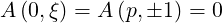
where the function A is such that the flux of electrons between two contours A1 and A2 is
equal to ne
is such that the flux of electrons between two contours A1 and A2 is
equal to ne
 . Lets consider a path γ12 between the contours A1 and A2. The total
flux of electrons through this path, which is in fact a surface, given the rotational symmetry in
φ, is given by
. Lets consider a path γ12 between the contours A1 and A2. The total
flux of electrons through this path, which is in fact a surface, given the rotational symmetry in
φ, is given by
| Γ12 | =  S12dSSp ⋅ S12dSSp ⋅ | ||
=  S12dS ⋅∇× Tφ S12dS ⋅∇× Tφ | |||
= ∮
 12Tφdl ⋅ 12Tφdl ⋅ | (3.337) |
By rotational symmetry in φ, and using (A.272), we get
 | (3.338) |
If we define
 | (3.339) |
we obtain
 | (3.340) |
and therefore the total flux between the contours A1 and A2 is equal to ne
 . We
call A
. We
call A the stream function, and we get finally
| Sp | =   | (3.341) |
| Sξ | =   | (3.342) |
Since there are no fluxes across the internal boundaries in the momentum space, this boundary coincide with a contour A, and therefore we can arbitrarily set this value to 0:
 | (3.343) |
Then A can be calculated by any of the integrals
 | (3.344) |
or
 | (3.345) |
However, A remains a function of ξ, which depends upon θ. Starting from the
bounce-averaged fluxes, it is interesting to compute a function A
remains a function of ξ, which depends upon θ. Starting from the
bounce-averaged fluxes, it is interesting to compute a function A
 , such
that
, such
that
A  | = A = 0 = 0 | ||
Sp | =   | (3.346) | |
Sξ | =   |
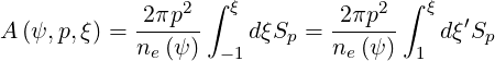
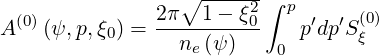
We first need to demonstrate the existence of such a function. Starting from Sp ,
,
A  | =  ∫
-1ξ0
dξ0′ ∫
-1ξ0
dξ0′ | ||
=  ∫
-1ξ0
dξ0′ ∫
-1ξ0
dξ0′ ![[ ∑ ]
1-
2 σ](NoticeDKE1081x.png) T ∫
θminθmax T ∫
θminθmax
     Sp Sp | |||
= ∫
-1ξ0
dξ0′ ![[ ]
1-∑
2
σ](NoticeDKE1088x.png) T ∫
02π T ∫
02π H H      | |||
=  ![[ ∑ ]
1-
2 σ](NoticeDKE1097x.png) T ∫
02π T ∫
02π    | |||
∫
-1ξ0
dξ0′H σ σ  | |||
=  ![[ ]
1∑
2
σ](NoticeDKE1106x.png) T ∫
02π T ∫
02π     ∫
-1ξdξ′ ∫
-1ξdξ′ | |||
=  ![[ ∑ ]
1-
2 σ](NoticeDKE1114x.png) T ∫
02π T ∫
02π    σA σA | |||
= σ ![[ ]
1∑
2
σ](NoticeDKE1120x.png) T T  V V | (3.347) |
where we used
 | (3.348) |
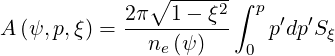
Now, starting from Sξ , we have
A  | =  ∫
0pp′dp′σ ∫
0pp′dp′σ | ||
=  ∫
0pp′dp′σ ∫
0pp′dp′σ ![[ ]
1-∑
2
σ](NoticeDKE1130x.png) T ∫
θminθmax T ∫
θminθmax
     Sξ Sξ | |||
= ∫
0pdp′σ ![[ ∑ ]
1-
2 σ](NoticeDKE1137x.png) T ∫
θminθmax T ∫
θminθmax
       | |||
=  ![[ ]
1∑
2
σ](NoticeDKE1146x.png) T ∫
θminθmax T ∫
θminθmax
     ∫
0pdp′ ∫
0pdp′ | |||
=  ![[ 1∑ ]
--
2 σ](NoticeDKE1154x.png) T ∫
θminθmax T ∫
θminθmax
    σA σA | |||
= σ ![[ ]
1-∑
2
σ](NoticeDKE1160x.png) T T  V V | (3.349) |
and we find the same function A . The existence of a function A
 verifying (3.346) is
therefore demonstrated. We need now to demonstrate that A
verifying (3.346) is
therefore demonstrated. We need now to demonstrate that A verifying (3.346) leads to the
bounce-averaged Fokker-Planck equation (3.166):
verifying (3.346) leads to the
bounce-averaged Fokker-Planck equation (3.166):
 | =    - -   | ||
=    - -   | |||
=   ![[ (0)]
λne(ψ-)A---
2π](NoticeDKE1180x.png) - -  ![[ (0)]
λne(ψ-)A---
2π](NoticeDKE1183x.png) | |||
| = 0 | (3.350) |
In conclusion, a stream function verifying
 | (3.351) |
has been found which leads to the bounce-averaged Fokker-Planck equation and which can be calculated from the bounce-averaged fluxes by either
 | (3.352) |
or
 | (3.353) |
relations.
The electrical conductivity of the plasma σe is defined as the ratio of the flux averaged current
density  ϕ0 to the flux surface averaged parallel Ohmic electric field
  ϕ,
ϕ,
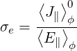 | (3.354) |
By definition,
 ϕ ϕ | =  ∫
02π ∫
02π    E∥ E∥ ![[ ]
ϕ^⋅^b](NoticeDKE1198x.png) | ||
=  ∫
02π ∫
02π    E∥ E∥  | |||
=  ∫
02π ∫
02π     | (3.355) |
Using
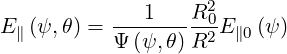 | (3.356) |
where E∥0 is the value at the minimum magnetic field B0, one obtains
 ϕ ϕ | =  ∫
02π ∫
02π      | ||
= E∥0  ∫
02π ∫
02π      | (3.357) |
or
 ϕ ϕ | = E∥0   ∫
02π ∫
02π     ![[ ]
ξ-BT-----1--- R30-
ξ0 B Ψ2 (ψ,θ) R3](NoticeDKE1241x.png) | ||
= E∥0   ∫
02π ∫
02π     × × | |||
![[ ξ BT BT 0B0 1 R3 ]
---------------2-------03
ξ0BT 0 B0 B Ψ (ψ,θ)R](NoticeDKE1250x.png) | |||
= E∥0    ∫
02π ∫
02π     ![[ ]
ξ-----1---R40
ξ0Ψ3 (ψ,θ)R4](NoticeDKE1260x.png) | |||
= E∥0    λσ λσ | |||
= E∥0    λ1,-3,4 λ1,-3,4 | (3.358) |
Case of circular concentric flux-surfaces In that case,
 | (3.359) |
and since Rp∕R0 = 1∕ ,
,
 ϕ ϕ | =  λ1,-1,2E∥0 λ1,-1,2E∥0 | ||
=  λ1,1,0E∥0 λ1,1,0E∥0 | (3.360) |
using relation Ψ = R∕R0. Therefore,
 | (3.361) |
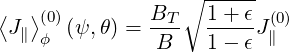
as λ1,-1,2 =  for circular concentric flux-surfaces. Moreover, in this limit,
 | (3.362) |
since
 | (3.363) |
with
 | (3.364) |
In that case, the neo-classical conductivity can be either calculated from flux surface averaged quantity, or local values at B = B0.
The ratio between the number of trapped and passing electrons is an important quantity in the neoclassical transport theory, since the parallel viscosity responsible for reduction of the Ohmic conductivity and the bootstrap current level are both roughly proportional to this parameter. Therefore, under the influence of RF waves, its large variation will indicate unambiguously that significant macroscopic changes are to be expected on the current generation and the power absorption due to neoclassical effects. We could expect to encounter such circomstances especially when wave-particle interaction takes place in the near vicinity of the trapped-passing boundary.
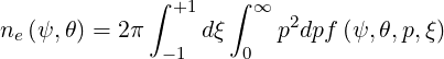
The starting point of the calculations is the determination of the flux averaged density  .
According to the definition of the electron momentum distribution function f, the local electron
density ne
.
According to the definition of the electron momentum distribution function f, the local electron
density ne is given by the relation
 | (3.365) |
Using the general expression (3.246) of the flux-surface averaging of a volumic quantity
 V V  | =  ∫
02π ∫
02π    ne ne | ||
=  ∫
0∞p2dp∫
02π ∫
0∞p2dp∫
02π    ∫
-1+1dξf ∫
-1+1dξf | |||
=  ∫
0∞p2dp∫
02π ∫
0∞p2dp∫
02π    × × | |||
∫
-1+1![[ ]
1-∑
2
σ=±1](NoticeDKE1306x.png) T dξf T dξf | (3.366) |
where the trapping condition evaluated at the location θ is given by
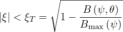 | (3.367) |
Using ξdξ = Ψξ0dξ0 with the condition (3.270) on ξ0
 | (3.368) |
one get
![∫ [ ] ∫ [ ] ( ∘ -----------)
+1 1-∑ +1 1- ∑ ξ0 ---1---
-1 2 dξ = -1 2 Ψ (ψ,θ) ξ H |ξ0|- 1 - Ψ (ψ,θ) dξ0
σ= ±1 T σ=±1 T](NoticeDKE1310x.png) | (3.369) |
Note that the condition (3.368) is equivalent to
 | (3.370) |
so that, the integrals over θ and ξ0 may be permuted,
 V V  | =  ∫
0∞p2dp∫
-1+1dξ
0× ∫
0∞p2dp∫
-1+1dξ
0× | ||
![[ ]
1-∑
2 σ=±1](NoticeDKE1315x.png) T ∫
θminθmax T ∫
θminθmax
     f f | (3.371) |
where the bounce-averaging of the distribution appears naturally. Therefore, expression (3.371) can be rewriten in the simple form
 | (3.372) |
and the exact trapped fraction  t is given by the ratio
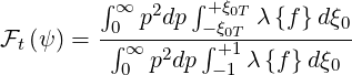 | (3.373) |
where λ is the normalized bounce time 2.11.
Since,  ≃ f0
≃ f0 +
+
 +g
+g ,
,
![∫∞ 2 ∫+ξ0T [ (0) (0)]
F (ψ) = ---0-p-dp---ξ0T[-λ--f0--+-g---d]ξ0---
t ∫∞ p2dp ∫+1 λ f(0)+ ^f(0) + g(0) dξ
0 -1 0 0](NoticeDKE1329x.png) | (3.374) |
taking into account that 
 is an odd function of ξ0 in the trapped region.
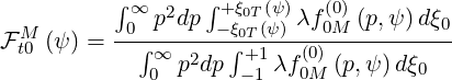
When f0 = f0M
= f0M = fM is a Maxwellian distribution on the magnetic flux surface
ψ,
= fM is a Maxwellian distribution on the magnetic flux surface
ψ,
![∫ ∫
∞0 p2dp +-ξξ0Tλf0(0M)dξ0
F Mt (ψ ) = ∫-∞----∫-+1--[0T(0)----(0)]----
0 p2dp -1 λ f0M + gM d ξ0](NoticeDKE1334x.png) | (3.375) |
taking into account that gM = 0 for trapped electrons. Neglecting the contribution of gM
 ,
the zero order trapped fraction t0M is given by
,
the zero order trapped fraction t0M is given by
 | (3.376) |
which reduces to
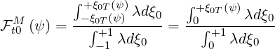 | (3.377) |
In this limit, t0M is only a function of the geometrical magnetic configuration, while is the
general case, t is a fully kinetic quantity.
Case of circular concentric flux-surfaces In that case, the normalized bounce time is simply
![∫ [ ]
θmaxdθ-ξ0 2- 1-2
λ (ξ0) = 2π ξ ≃ π J0(ξ0,ξ0T)- 2ξ0TJ2(ξ0,ξ0T )
θmin](NoticeDKE1339x.png) | (3.378) |
which may be expanded up to the second order with an excellent accuracy as shown in Appendix ??. Here,
 | (3.379) |
with ϵ = r∕Rp the usual inverse aspect ratio.
It is interesting to estimate the parametric dependence of t0M for ϵ ≪ 1. For trapped
particles,
![[ ( ) [ ( ) ( )]]
2|ξ0| -ξ02 1-2 -ξ20 -ξ20
λ(ξ0) ≃ πξ0T K ξ2 - 2ξ0T K ξ2 - E ξ2
0T 0T 0T](NoticeDKE1341x.png) | (3.380) |
where K and E
and E are complete elliptic integrals of the first and second kind.
Hence,
are complete elliptic integrals of the first and second kind.
Hence,
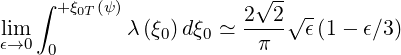
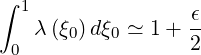
![∫ + ξ0T(ψ) 2√2-√ -∫ 1
λ(ξ0)dξ0 = ---- ϵ x[K (x)- ϵ(K (x )- E (x))]dx
0 π 0](NoticeDKE1344x.png) | (3.381) |
Using the recurrence relation
 | (3.382) |
and since
 | (3.383) |
according to formulaes (6.147) and  in Ref. [?],
 | (3.384) |
For circulating electrons,
![[ ( ) [ ( ) ( ) ]]
λ(ξ ) ≃ 2- K ξ20T - 1-ξ2 K ξ20T - E ξ20T
0 π ξ20 2 0 ξ20 ξ20](NoticeDKE1349x.png) | (3.385) |
and
 | (3.386) |
From the relation
 | (3.387) |
which is given by formula  of Ref. [?],
∫
+ξ0T 1λ 1λ dξ0 dξ0 | =    + +  ϵ ϵ ∫ ∫
 1 1 dx dx | ||
≃ 1 -  + +  ϵ ϵ ∫ ∫
 1 1 dx dx | (3.388) |
and using the indefinite integrals
 | (3.389) |
and
![∫ E (x ) 1 [ 2 ( 2) ]
-x4--dx = 9x3-2(x - 2)E (x)+ 1 - x K (x)](NoticeDKE1369x.png) | (3.390) |
according to formulaes (5.113.1) and  in Ref. [?],
 | (3.391) |
so that up to the first order term,
 | (3.392) |
Consequently,
 | (3.393) |
and the  dependence in the limit ϵ ≪ 1 is well recovered, as expected from an intuitive
explanation.
dependence in the limit ϵ ≪ 1 is well recovered, as expected from an intuitive
explanation.
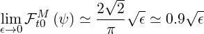
It is worth noting that this result is well recovered by a simple Monte-Carlo technique, where
the poloidal angle θ is taken to be a uniform random variable between 0 and 2π, as well as ξ
between -1 and 1. Using the relation (2.22) which translates ξ to ξ0 at the minimum B
value, and considering that the particle is trapped when  ≤ ξ0T , the fraction of
trapped particle found numerically is exactly t0M
≤ ξ0T , the fraction of
trapped particle found numerically is exactly t0M , while the distribution scales like
λ
, while the distribution scales like
λ .
.
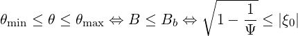
It is important to precise that t0M is not the “ effective” trapped fraction teff. given by
the well known relation
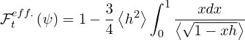 | (3.394) |
found repeatedly in the litterature for the bootstrap current or the neoclassical conductivity,
where h = B∕Bmax and Bmax is the maximum value of the magnetic field B along the particle
trajectory. This quantity results from the reduction of the conductivity due to trapped particles,
or the onset of the bootstrap current. Its expression with notations used in the text is
determined from the bootstrap current calculations with the Lorentz collision operator, as
shown Sec.5.6.2. It is important to notice that teff. is in principle not a fraction
of trapped electrons, and in addition there is no demonstration that teff. ≤ 1 is
always satisfied for all magnetic configurations, as mentioned clearly in Ref. [?]. In
fact the denomination “ effective” trapped fraction teff. is quite confusing, since
it applies only for Maxwellian regime, and is not established as a kinetic quantity
like t0M. This point is especially important when non-Maxwellian distributions are
considered for evaluating the bootstrap current. Consequently, teff. must not be used in
such regimes, but only t as an true physical sense for comparisons between different
regimes.
Primary generation When the Ohmic electric field E∥ exceeds the Dreicer level ED, a fraction of the electron population run away. The total number of electrons is therefore no more conserved, since the flux Sp≠0 at p = pmax, on the boundary of the integration domain ϒ. The runaway loss rate ΓR is given by the relation
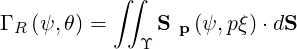 | (3.395) |
where the element of surface dS = p2dξdφ
 according to the Appendix A. Therefore, since
∫
dφ = 2π by symmetry, one obtains
according to the Appendix A. Therefore, since
∫
dφ = 2π by symmetry, one obtains
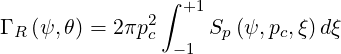 | (3.396) |
where pc is the critical momentum above which electrons runaway. The value of pc corresponds
to the threshold where collision drag may not counter-balance electric field acceleration, and its
value is therefore dependent of the model used for collisions. Since electrons with p ≥ pc will
never cross back this threshold, they leave rapidly the domain of integration, and
ΓR is weakly dependent of p when p ≥ pc. In particular, ΓR
 ≈ ΓRmax
 ,
where
,
where
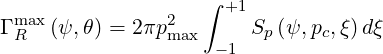 | (3.397) |
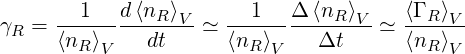
Consequently, pc is considered as a free parameter in the code. The flux-surface averaged
runaway rate  V is given by the relation
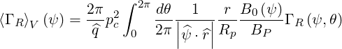 | (3.398) |
or
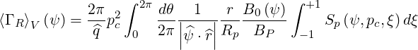 | (3.399) |
Using the usual condition on the trapped electrons,
 | (3.400) |
one obtains
 V V  | =  pc2 ∫
-1+1dξ
0 pc2 ∫
-1+1dξ
0![[ ]
1 ∑
2-
σ](NoticeDKE1394x.png) T ∫
θminθmax T ∫
θminθmax
     Sp Sp | ||
=  pc2 ∫
-1+1 pc2 ∫
-1+1 λ λ   dξ0 dξ0 | |||
=  2πpc2 ∫
-1+1λ 2πpc2 ∫
-1+1λ Sp Sp  dξ0 dξ0 | (3.401) |
since the sum ![[1∑ ]
2 σ](NoticeDKE1410x.png) T may be added, because Sp
T may be added, because Sp does not depend of the sign of ξ. in
the trapped region. The density Δ
does not depend of the sign of ξ. in
the trapped region. The density Δ V of runaway electrons lossed per time step Δt is then
simply
V of runaway electrons lossed per time step Δt is then
simply  V
V  Δt, and in order to preserve the code conservative, a source of thermal
electrons corresponding to a similar amount of electrons lost must be added in the set of
equations to solve.
Δt, and in order to preserve the code conservative, a source of thermal
electrons corresponding to a similar amount of electrons lost must be added in the set of
equations to solve.
Secondary generation The Fokker-Planck approximation for collisions is valid so far electrons suffer only weak deflections. Knock-on processes are consequently neglected. However, for electrons with a high kinetic energy p ≳ lnΛ†, such an approximation is no more justified, and collisions with large deflections must be considered. The effect may change significantly the picture of the fast tail build-up by leading to an avalanche process that could modify the runaway electron growth rate
 | (3.402) |
Here  V is the flux surface averaged runaway density.
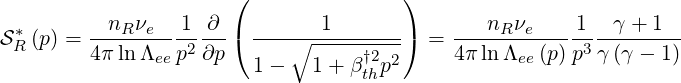
The source  R of secondary runaway electrons is given by a Krook term of the form [?]
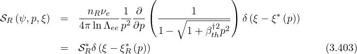
 | (3.404) |
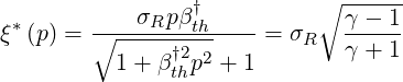
is the pitch-angle of the secondary electron produced by collisions, which is here deduced from momentum and energy conservation of strong elastic collisions between relativistic particles (See Appendix ?? )1, and
 | (3.405) |
Here, γ =  and the normalized density of runaway electrons nR is assumed to be
uniform over a magnetic flux surface ψ, so that nR = nR
and the normalized density of runaway electrons nR is assumed to be
uniform over a magnetic flux surface ψ, so that nR = nR =
=  V , lnΛee is the usual
Coulomb logarithm for electron-electron collisions, which is a function of p for high
energy electrons, and σR = v∥∕v indicates the direction of acceleration for the runaway
electrons.
V , lnΛee is the usual
Coulomb logarithm for electron-electron collisions, which is a function of p for high
energy electrons, and σR = v∥∕v indicates the direction of acceleration for the runaway
electrons.
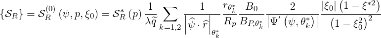
The bounce-averaged expression of R is given by the usual relation
![[ ∑ ] ∫ θmax
{SR } = -1- 1- dθ-|-1-|-r--B- ξ0SR (ψ,p,ξ)
λ^q 2 σ θmin 2π ||ψ^⋅^r||Rp BP ξ
T](NoticeDKE1423x.png) | (3.406) |
or
![[ ∑ ] ∫ θmax
{SR} = S*R (p) 1-- 1- dθ|--1-|-r--B- ξ0-δ(ξ - ξ*)
λ^q 2 σ T θmin 2π||ψ^⋅^r||Rp BP ξ
* *
= SR (p) {δ(ξ - ξ )} (3.407)](NoticeDKE1424x.png)
In order to calculate  , it is important to recall that ξ is a function of θ, according
to the relation
, it is important to recall that ξ is a function of θ, according
to the relation
 | (3.408) |
where Ψ = B
= B ∕B0
∕B0 . Using the general relation δ
 = ∑
kδ
= ∑
kδ ∕
∕ for the Delta function δ
 , where xk are the zeros of function g
 and g′
 = dg∕dx, one
obtains
= dg∕dx, one
obtains
 | (3.409) |
where θk* are the poloidal angle values where the secondary electron emerges, which verify the relation
 | (3.410) |
or
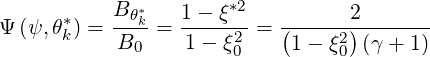 | (3.411) |
Indeed, the equation Ψ = C has in general two distinct solutions in a tokamak magnetic
configuration, except at θ* =
= C has in general two distinct solutions in a tokamak magnetic
configuration, except at θ* =  . Therefore,
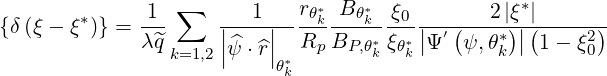
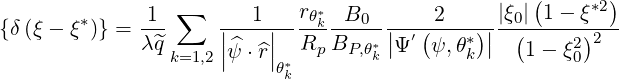
![[ ] ∫ θ *
{δ (ξ - ξ*)} =-1- 1-∑ max dθ-|-1-|-r--B- ξ0 ∑ |--(---2|)ξ|(|-----)δ(θ - θ*)
λ^q 2 σ θmin 2π ||ψ^⋅^r||Rp BP ξ |Ψ′ ψ,θ*k | 1 - ξ20 k
T k=1,2](NoticeDKE1441x.png) | (3.412) |
or
 | (3.413) |
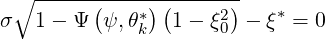
since the integrand is an even function of ξ (or ξ0). Consequently
 | (3.414) |
or
 | (3.415) |
since
 | (3.416) |
Finally,
 | (3.417) |
and using relations 3.405 and 3.404,
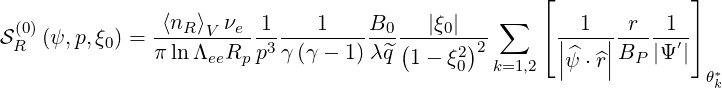 | (3.418) |
where  V = ∫
-∞t
V = ∫
-∞t V dt corresponds to the total number of runaway electrons produced
at the normalized time t on a flux surface ψ.
V dt corresponds to the total number of runaway electrons produced
at the normalized time t on a flux surface ψ.
The flux-surface averaged source term  V is given by the general relation
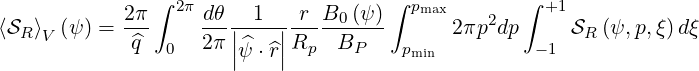 | (3.419) |
which becomes
 | (3.420) |
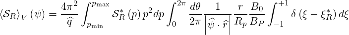
or
 | (3.421) |
Since by definition ∫
-1+1δ dξ = 1, and using the relation
 | (3.422) |
one finds
 | (3.423) |
or
 | (3.424) |
assuming a weak dependence of lnΛee with p in the interval of integration.
Recalling that nR =  V , the relation between the normalized secondary runaway source
and the runaway rate is then simply
V , the relation between the normalized secondary runaway source
and the runaway rate is then simply
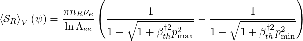
 | (3.425) |
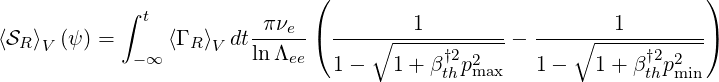
where values pmin and pmax correspond respectively to the runaway threshold pc and the upper momentum boundary of the integration domain of the Fokker-Planck equation. An estimate of pmin is given in Appendix ??. In the limit βth†2pmax2 ≫ 1,
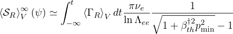 | (3.426) |
and using the relation βth†2pmin2 ≈ 2Ec∕E∥ when E∥≫ E*, where E* is the critical electric field for relativistic electrons,
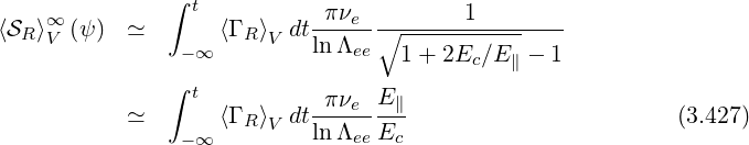
Using relation
 | (3.428) |
between Dreicer field ED and the critical electric field Ec, one obtains finaly when E∥∕ED ≫ βth†2,
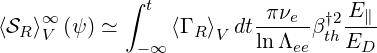 | (3.429) |
A similar expression may be derived in the opposite limit, i.e. when E∥≳ Ec or E∥∕ED ≳ βth†2. In that case,
 | (3.430) |
Λeeand
 | (3.431) |
Since the secondary source term will enhance the fast electron density above pmin, for a
given electric field, the effect of strong Coulomb collisions will greatly increase the loss
of runaway electrons. The fact that  V ∞ is not proportional to
  V but to
∫
-∞t
V but to
∫
-∞t V dt clearly indicates that all the history of the fast tail build-up plays a
crucial role on the dynamics at time t, and consequently, only a time evolution is
meaningful for this studying this problem which has basically no stationnary regime. A
stationnary regime may only be found if E∥ evolves so that the plasma current is kept
time-independent.
V dt clearly indicates that all the history of the fast tail build-up plays a
crucial role on the dynamics at time t, and consequently, only a time evolution is
meaningful for this studying this problem which has basically no stationnary regime. A
stationnary regime may only be found if E∥ evolves so that the plasma current is kept
time-independent.
Though magnetic ripple losses is a full 4 -D problem, it can be considered in a simple manner by defining a super-trapped volume V ST p in momentum space,
 | (3.432) |
in which particle escape the plasma. A low energy, it is bounded by the collision detrapping when p ≤ pc, while the pitch-angle dependence results from the condition that only electrons whose banana tip enter the bad confinement region characterized by the well known criterion α*≤ 1 are trapped in the magnetic well, in an irreversible manner. As shown in Fig. 3.1, even if this is a rather crude modeling, it captures most of the salient features of the physics. Therefore, all trapped electrons which in addition fullfils the condition p∥∕p ≤ ξ0ST are super-trapped. Here, ξ0ST is deduced from the intersection between the poloidal extend of the banana and the good confinement domain α* ≥ 1 on a given flux surface [?]. The pitch-angle threshold ξ0ST depends therefore of the radial position ψ and close to the edge,
 | (3.433) |
which indicates that all trapped electrons are expected to escape the magnetic configuration. Furthermore, it is assumed that electrons, once in this magnetic well, do not contribute anymore to the overall momentum dynamics, which is obviously a very crude approximation.
cmcmcm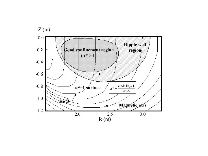
An heuristic description of this process may be obtained by introducing a Krook term restricted to the volume V ST p in the Fokker-Planck equation
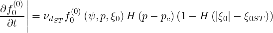 | (3.434) |
where νdST-1 is the drifting time taken by super-trapped electrons for leaving the plasma. In
order to reproduce the fact that super-trapped electrons are decoupled from the momentum
dynamics, a simple method is to force νdST-1 ≪ τb. Without detailed knowledge
of the local dynamics, νdST is taken constant in V ST p, which is obviously a coarse
approximation. However, in the limit νdST-1 ≪ τb, the shape of the distribution function
becomes independent of νdST, since by definition f0
 ≃ 0 in the super-trapped
domain.
≃ 0 in the super-trapped
domain.
Obviously, when a Krook term is introduced, the Fokker-Planck equation is no more conservative, since a fraction of fast electrons is definitively leaving the plasma . Assuming the particle loss rate is small, a steady-state solution may be found, provided some external source of electron is added, in order to keep the density locally constant. This important point is discussed in Sec.5.7.1. The new form of the bounce-averaged Fokker-Planck equation is
 | (3.435) |
and in this stationnary limit limt→∞∂f0 ∕∂t = 0,
 | (3.436) |
Losses are assumed to be mainly local, since they occur on a very short time scale as compared to the fast electron transport one. Therefore, only the momentum dynamics is considered, and integrating equation (3.436 ), one obtains
 V STp∇ V STp∇ ⋅ Sp ⋅ Sp J
pJξ0dpdξ0dφ J
pJξ0dpdξ0dφ | |||
= - V STpνdSTf0 V STpνdSTf0 H H 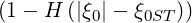 JpJξ0dpdξ0dφ JpJξ0dpdξ0dφ | (3.437) |
where Jp and Jξ
0are the Jacobians as defined in Sec. 3.5.1. The magnetic ripple loss rate
ΓST 
 on the B0 axis is simply given by
 | (3.438) |
or
 | (3.439) |
since ∫ dφ = 2π.
An equivalent form can be deduced from the flux of particle leaving the integration domain,
ΓST   | =  V STp∇ V STp∇ ⋅ Sp ⋅ Sp J
pJξ0dpdξ0dφ J
pJξ0dpdξ0dφ | ||
=  SSTpSp SSTpSp ⋅ dS ⋅ dS | (3.440) |
using the Green-Ostrogradsky theorem, where SST p is the surface that encloses volume V ST p. as shown in Fig. 3.1, SST p may be split into two terms corresponding to coordinate surfaces
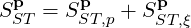 | (3.441) |
where SST,pp is the surface at constant p, while SST,ξ0p is the surface at constant ξ0 . Therefore, for the surface SST,pp,
 | (3.442) |
 | (3.443) |
according to the differential relations in Appendix A. One obtains finaly
 | (3.444) |
since the flux Sξ0 is a symmetric function of ξ0.
According to adjoint formalism developped by P. Helander [?], the flux surface averaged cross-field particle flux may be expressed as
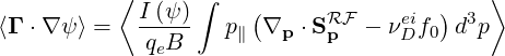 | (3.445) |
where  = RBT , and the Coulomb deflection frequency νDei is given by the
relation
= RBT , and the Coulomb deflection frequency νDei is given by the
relation
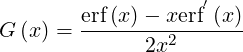
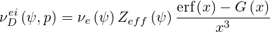 | (3.446) |
with x = p∕ and
and
 | (3.447) |
Expression (3.445) is only valid in the non-relativistic limit, i.e. when βth†≪ 1.
From the expression of the flux divergence ∇p ⋅ Sp

 | (3.448) |
one obtains
![[ ]
∫ RF 3 ∫ ∞ ∫ +1 ∂ ( 2 RF) 2 ∂ (∘ ------ RF )
p∥∇p ⋅Sp d p = 2π dp ξ p ∂p-p S p - p ∂ξ- 1 - ξ2Sξ dξ
0 - 1](NoticeDKE1506x.png) | (3.449) |
where
![∫ ∞ ∫ +1 ∂ (∘ ------ )
- 2π dp ξp2--- 1- ξ2SRFξ dξ
∫ 0 -1( ∂ξ ∫ )
∞ 2 [ ∘ ----2-RF ]+1 +1 ∘ ----2- RF
= - 2π 0 pdp ξ 1- ξ Sξ -1 - -1 1- ξ Sξ dξ
∫ ∞ ∫ +1 ∘ ------
= 2π p2dp 1 - ξ2SRξF dξ
0 - 1
∫ +1∘ ------ ∫ ∞ 2 RF
= 2π 1 - ξ2dξ pS ξ dp (3.450)
-1 0](NoticeDKE1507x.png)
![∫ ∞ ∫ +1 ∂ ( ) ∫ +1 ∫ ∞ ∂ ( )
2π dp ξp--- p2SRpF dξ = 2π ξdξ p --- p2SRFp dp
0 -1 ∂p ∫- 1 (0 ∂p ∫ )
+1 [ 3 RF ]∞ ∞ 2 RF
= 2π - 1 ξdξ p Sp 0 - 0 p Sp dp
∫ +1 ∫ ∞
= - 2π ξd ξ p2SRpF dp (3.451)
-1 0](NoticeDKE1508x.png) = 0. It is important to recall that this condition is more stringent
than the equivalent one for RF power calculation, where the condition limp→∞p2Sp = 0 must
hold.
= 0. It is important to recall that this condition is more stringent
than the equivalent one for RF power calculation, where the condition limp→∞p2Sp = 0 must
hold.
Therefore
 | (3.452) |
and finally
![∫
( RF ei ) 3
p∥ ∇p ⋅S p - νD (p)f0 d p
∫ +1∘ ------ ∫ ∞ ∫ +1 ∫ ∞ [ ]
= 2π 1- ξ2dξ p2SRξF dp- 2 π ξdξ p2 SRpF + νeDipf0 dp(3.453)
-1 0 - 1 0](NoticeDKE1510x.png)
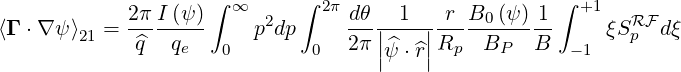
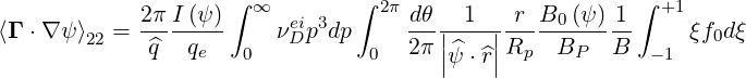
Since  is a volume quantity, the flux surface averaged expression (3.445) may be
then expressed as
is a volume quantity, the flux surface averaged expression (3.445) may be
then expressed as
 | (3.454) |
where
 | (3.455) |
![∫ 2π ∫ +1 ∫ ∞
⟨Γ ⋅∇ ψ⟩ = 2π-I (ψ-) dθ|--1-|-r-B0-(ψ)-1 ξdξ p2[SRF + νei(p)pf]dp
2 ^q qe 0 2π||^ψ ⋅^r||Rp BP B -1 0 p D](NoticeDKE1514x.png) | (3.456) |
Expressions  1 and
1 and  2 must be expressed in terms of bounce-averaged
quantities so that calculations may be performed numerically in the code. By permuting
integrals,
2 must be expressed in terms of bounce-averaged
quantities so that calculations may be performed numerically in the code. By permuting
integrals,
 | (3.457) |
and since  Sξ is an even function of ξ for trapped electrons, it is equivalent
to
Sξ is an even function of ξ for trapped electrons, it is equivalent
to
![∫ ∞ ∫ 2π [ ∑ ] ∫ +1∘ ------
⟨Γ ⋅∇ψ ⟩ = 2-πI-(ψ-) p2dp -dθ|-1--|-r-B0-(ψ)-1 1- 1 - ξ2SRF dξ
1 ^q qe 0 0 2π ||^ψ ⋅^r||Rp BP B 2 σ=±1 -1 ξ
T](NoticeDKE1519x.png) | (3.458) |
Using ξdξ = Ψξ0dξ0 with the condition (3.270) on ξ0
 | (3.459) |
we get that
 | (3.460) |
which is equivalent to
 | (3.461) |
Therefore,
![2πI (ψ)∫ ∞ 2 ∫ 2π dθ 1 r B0 (ψ) 1
⟨Γ ⋅∇ ψ⟩1 = ^q---q-- pdp 2-π||^---||R---B----B-
e 0 0 |ψ ⋅^r| p P
[ ∑ ] ∫ +1∘ ------ ( ∘ -----------)
× 1- 1 - ξ2Ψ3∕2ξ0H |ξ0|- 1- ---1--- SRF(d3ξ.4062)
2σ= ±1 -1 0 ξ Ψ (ψ, θ) ξ
T](NoticeDKE1523x.png)
![∫ ∫
2π---I (ψ)- ∞ 2 +1 ∘ ----2-
⟨Γ ⋅∇ ψ⟩1 = ^q qeB0 (ψ) p dp dξ0 1- ξ0
[ ] ∫0 -1 ( )2
1-∑ θmax dθ|-1--|-r--B-ξ0 B0(ψ-) 3∕2 RF
× 2 θmin 2π|^ψ ⋅^r|Rp BP ξ B Ψ Sξ (3.463)
σ=±1 T | |](NoticeDKE1524x.png)
![∫ ∞ ∫ +1 ∘ ------[ ] ∫ θ
⟨Γ ⋅∇ψ ⟩ = 2-π--I (ψ-) p2dp dξ 1- ξ2 1-∑ max dθ-|-1-|-r--B- ξ0Ψ- 1∕2SRF
1 ^q qeB0 (ψ) 0 -1 0 0 2 θmin 2π ||ψ^⋅^r||Rp BP ξ ξ
σ=±1 T](NoticeDKE1525x.png) | (3.464) |
which is equivalent to
 | (3.465) |
where we use the bounce-averaged definition
![{ } [ ∑ ] ∫ θmax
Ψ -1∕2SRF = -1- 1- -dθ|-1--|-r--B-ξ0Ψ -1∕2SRF
ξ λ ^q 2σ=±1 θmin 2 π||^ψ ⋅^r||Rp BP ξ ξ
T](NoticeDKE1527x.png) | (3.466) |
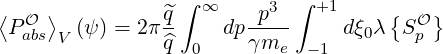
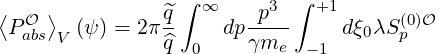
Much in the same way,
 | (3.467) |
where
 | (3.468) |
and
 | (3.469) |
Applying the same technique as for  1, using the fact that Sp
 = Sp
= Sp in
the trapped region, one obtains
in
the trapped region, one obtains
![2π I (ψ )∫ ∞ ∫ 2πdθ 1 r B0 (ψ )1
⟨Γ ⋅∇ ψ⟩21 = -------- p2dp ---||----||-----------
^q qe 0 0 2π |^ψ ⋅^r|Rp BP B
[ ] ∫ +1 ( ∘ -----------)
× 1- ∑ Ψξ H |ξ |- 1- ---1--- SRF dξ (3.470)
2 - 1 0 0 Ψ (ψ, θ) p 0
σ=±1 T](NoticeDKE1534x.png)
 | (3.471) |
since the integrand is odd in ξ0, and
![{ } [ ∑ ] ∫ θmax ( )
σ ξ-Ψ- 1SRF = -1- 1- dθ-|-1--|r--B--ξ0 σ-ξΨ -1SRF
ξ0 p λ^q 2 σ=±1 θmin 2π ||^ψ ⋅ ^r||Rp BP ξ ξ0 p
[ ]T
1 1 ∑ ∫ θmaxdθ 1 r B0 RF
= λ^q- 2- 2π-||^---||R--B--σSp (3.472)
σ=±1 T θmin |ψ ⋅ ^r| p P](NoticeDKE1536x.png)
In a similar way,
![2π I (ψ )∫ ∞ ei 3 ∫ 2π dθ 1 r B0 (ψ) 1
⟨Γ ⋅∇ψ ⟩22 = -^q--q--- νD p dp 2π||^---||R----B---B-
e 0 0 |ψ ⋅^r| p P
[ ∑ ] ∫ +1 ( ∘ -----------)
× 1- Ψξ0H |ξ0|- 1- ---1--- fdξ (3.473)
2 σ=±1 -1 Ψ (ψ, θ)
T](NoticeDKE1537x.png)
 | (3.474) |
and an even function in ξ0 for trapped electrons, one obtains
 | (3.475) |
or
 | (3.476) |
Finally, it is necessary to evaluate σ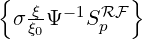 and
and  from the quasilinear
diffusion coefficients. Starting from the conservative form of the wave-induced fluxes in
momentum space
from the quasilinear
diffusion coefficients. Starting from the conservative form of the wave-induced fluxes in
momentum space
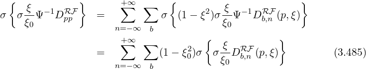
Using diffusion coefficients (4.233-4.236) defined in Sec. 4.3,
| Dpp | = ∑
n=-∞+∞∑
b(1 - ξ2)D
b,n(p,ξ) | (3.481) |
| Dpξ | = ∑
n=-∞+∞∑
b - ![[ 2 nΩ ]
1- ξ - ω--
b](NoticeDKE1547x.png) Db,n(p,ξ) Db,n(p,ξ) | (3.482) |
| Dξp | = ∑
n=-∞+∞∑
b - ![[ ]
1- ξ2 - nΩ-
ωb](NoticeDKE1549x.png) Db,n(p,ξ) Db,n(p,ξ) | (3.483) |
| Dξξ | = ∑
n=-∞+∞∑
b ![[ nΩ ]
1 - ξ2 - ---
ωb](NoticeDKE1551x.png) 2D
b,n(p,ξ) 2D
b,n(p,ξ) | (3.484) |
one obtains
![{ } { ∘ ------ [ ] }
ξ2 -3∕2 RF +∑ ∞ ∑ --1--ξ2-ξ2 - 3∕2 2 nΩ- RF
ξ2Ψ Dpξ = - ξ ξ2Ψ 1- ξ - ωb D b,n (p,ξ)
0 n= -∞ b ∘ ------ 0
+∑ ∞ ∑ 1 - ξ2[ n Ω0] { ξ }
= - -------0 1 - ξ20 ----- σ σ --DRbF,n (p,ξ) (3.486)
n= -∞ b ξ0 ωb ξ0](NoticeDKE1553x.png)
![{ } +∑ ∞ ∑ { ∘1---ξ2-[ nΩ ] }
DRFξp Ψ -1∕2 = - -------- 1- ξ2 - --- Ψ-1∕2DRFb,n (p,ξ)
n=- ∞ b ξ ωb
+∑ ∞ ∑ ∘ -----2[ ] { }
= - --1---ξ0 1 - ξ2- n-Ω0 σ σξ0 ΨDRF (p,ξ)(3.487)
n=- ∞ b ξ0 0 ωb ξ b,n](NoticeDKE1554x.png)
![{ }
{ ξ -1 RF } +∑ ∞ ∑ 1 [ 2 nΩ ]2 ξ -1 RF
σ σξ-Ψ D ξξ = σ σ ξ2 1 - ξ - ω-- ξ-Ψ D b,n (p,ξ)
0 n=- ∞ b b 0
+∑ ∞ ∑ 1 [ nΩ ]2 { ξ }
= -2 1- ξ20 - ---0 σ σ-0ΨDRFb,n (p,ξ) (3.488)
n=- ∞ b ξ0 ωb ξ](NoticeDKE1555x.png)
 depends only from
  b,nRF(0)D(p,ξ0) already defined for the
wave-induced bootstrap current in Sec.4.3, while
b,nRF(0)D(p,ξ0) already defined for the
wave-induced bootstrap current in Sec.4.3, while  depends from a quantity that is
very similar to
depends from a quantity that is
very similar to  b,nRF(0)F(p,ξ0). Using definitions
 b,nRF(0)D(p,ξ
0) b,nRF(0)D(p,ξ
0) | = σ | (3.489) |
 b,nRF(0)F(p,ξ
0) b,nRF(0)F(p,ξ
0) | = σ | (3.490) |
one obtains finally
 | (3.491) |
![{ 2 } +∑∞ ∑ ∘ -----2 [ ]
ξ2Ψ -3∕2DRpFξ = ---1---ξ0 1- ξ20 - nΩ0- D^RFb,n(0)D (p,ξ0) = ^DRFpξ (0)
ξ0 n=-∞ b ξ0 ωb](NoticeDKE1565x.png) | (3.492) |
and
![{ } +∑∞ ∑ ∘1---ξ2-[ nΩ ] ( { ξ })
DRFξp Ψ- 1∕2 = - ------0- 1- ξ02- ---0 D^RFb,n(0)F(p,ξ0)+ σ σ-0DRFb,n(p,ξ)
n=- ∞ b ξ0 ωb ξ
^ RF(0) ^RF,1(0)
= D ξp + D ξp (3.493)](NoticeDKE1566x.png)
![{ } +∑ ∞ ∑ [ ]2( { })
σ σ ξ-Ψ-1D ξξRF = -1 1- ξ02- nΩ0- ^DRF (0)F(p,ξ0)+ σ σ ξ0DRFb,n(p,ξ)
ξ0 n= -∞ b ξ20 ωb b,n ξ
RF (0) RF,1(0)
= D^ξξ + D^ξξ (3.494)](NoticeDKE1567x.png)
![∘ ------[ ] { }
RF,1(0) +∑∞ ∑ --1---ξ20 2 nΩ0- ξ0 RF
^D ξp = - ξ 1 - ξ0 - ω σ σ ξ D b,n(p,ξ)
n=-∞ b 0 b](NoticeDKE1568x.png) | (3.495) |
and
![+∑∞ ∑ 1 [ nΩ ]2 { ξ }
^DRFξ,ξ1 (0) = -2 1 - ξ20 - --0- σ σ 0-DRbF,n (p,ξ)
n=-∞ b ξ0 ωb ξ](NoticeDKE1569x.png) | (3.496) |
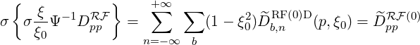
The bounce-averaged quasilinear diffusion coefficient σ may be easily
deduced from calculations of the RF wave-induced bootstrap current
may be easily
deduced from calculations of the RF wave-induced bootstrap current
![{ ξ0 RF } γpTe 1 rθbB θbξ30--RF,θb
σ σ ξ-Db,n (p,ξ) = p|ξ|λ-^qR----θbξ3D b,n,0 ×
0 pB P θb [ ]
1 ∑ ( θ ) || b,(n)||2
H (θb - θmin)H (θmax - θb)σ 2- σδ Nb∥ - N ∥bres |Θ(k3,θ.4b9|7)
σ T](NoticeDKE1571x.png)
Several other moments of the electron distribution function may be calculated, mainly for
diagnosing purposes of the plasma performances. In most cases, the local value of the
distribution function f must be determined not only at different plasma radius, but also
at various poloidal positions. In that case, the problem is 4 - D, since its shape is
function also of the poloidal position on a given flux surface ψ. A good example is the
calculation of the non-thermal bremsstrahlung [?], which requires the exact shape of the
distribution function f at each plasma position along the lines-of-sight, as well as the local
angle between the magnetic field line direction  and the direction of observation
 .
.
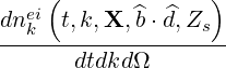
The number of counts NE0 that is recorded by a photon detection system in the energy range E0 ± ΔE between times tmin and tmax is given by the integral
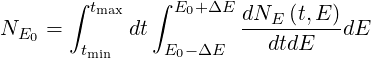 | (3.498) |
where dNE ∕dtdE is the measured photon energy spectrum. Its relation to the effective
photon energy spectrum dNk
∕dtdE is the measured photon energy spectrum. Its relation to the effective
photon energy spectrum dNk ∕dkdt emitted by the plasma in the direction of the detector
may be expressed as
∕dkdt emitted by the plasma in the direction of the detector
may be expressed as
 | (3.499) |
where G is the normalized instrumental response function,
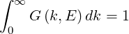 | (3.500) |
which gives the overall broadening of the energy spectrum, ηA the fraction of photons that
transmitted rather than being absorbed by various objects along the line-of-sight between the
plasma and the detector, and finally, 1 - ηD
the fraction of photons that
transmitted rather than being absorbed by various objects along the line-of-sight between the
plasma and the detector, and finally, 1 - ηD the fraction that are effectively stopped inside
the active part of the photon detector. For most detection systems, G
the fraction that are effectively stopped inside
the active part of the photon detector. For most detection systems, G is a complicated
function, that is usualy determined experimentaly with monoenergetic photon sources. It
incorporates the photoelectric conversion process that may be usualy modeled by a Gaussian
shape around the photon energy k whose half-width depends of the type of detector, and the
Compton scattering by electrons, which can be approximately described by a Fermi-like
function2.
is a complicated
function, that is usualy determined experimentaly with monoenergetic photon sources. It
incorporates the photoelectric conversion process that may be usualy modeled by a Gaussian
shape around the photon energy k whose half-width depends of the type of detector, and the
Compton scattering by electrons, which can be approximately described by a Fermi-like
function2.
Since the plasma is an extended source of photons, all contributions inside the volume ΔV viewing the detector with a solid angle ΔΩ must be added
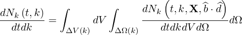 | (3.501) |
taking into account that photon plasma emissivity depends not only of the plasma position X
(inhomogeneity) but also of the angle  ⋅
⋅ between the directions of the magnetic field line
  X
and the line-of-sight
X
and the line-of-sight  at X (anisotropy that results from relativistic effects). In principle, both
ΔV
at X (anisotropy that results from relativistic effects). In principle, both
ΔV  and ΔΩ
 are functions of the photon energy, because of the partial transparency of
the collimating aperture with k. However, the design of the diaphragm is usualy optimized so
that this effect can be neglected.
are functions of the photon energy, because of the partial transparency of
the collimating aperture with k. However, the design of the diaphragm is usualy optimized so
that this effect can be neglected.
In the limit where the aperture of the diaphragm is small, so that variation of the photon
emissivity transverse to the line-of-sight may be neglected in the field of observation,
dNk ∕dtdk may be approximated by the simple sum
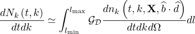 | (3.502) |
where Lc = lc max - lc min is the chord length in the plasma, and 
 is
a geometrical factor that is independent of the position lc along the
line-of-sight3.
Here, nk = dNk∕dV is the photon density. By definition, the determination of dNk
is
a geometrical factor that is independent of the position lc along the
line-of-sight3.
Here, nk = dNk∕dV is the photon density. By definition, the determination of dNk ∕dtdk
requires to evaluate X and
∕dtdk
requires to evaluate X and  X ⋅
X ⋅ as a function of l for a given magnetic equilibrium. Since
magnetic flux surfaces are nested in tokamaks inside the separatrix, the calculation requires the
determination of ψ
as a function of l for a given magnetic equilibrium. Since
magnetic flux surfaces are nested in tokamaks inside the separatrix, the calculation requires the
determination of ψ , θ
, θ and
and  ⋅
⋅ = cosθd
 .
.
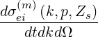
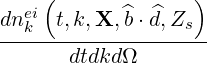
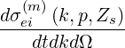
In the appropriate range of energy, the photon density energy spectrum results from the bremsstrahlung process only4. It is the sum of two contributions, one arising from electron-ion interactions, the other resulting from electron self-collisions
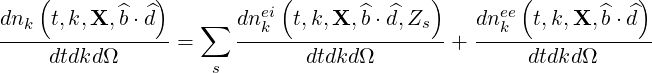 | (3.503) |
which are related to the respective bremsstrahlung differential cross-sections dσei/dtdkdΩ and dσee∕dtdkdΩ by the relations
 | (3.504) |
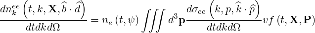 | (3.505) |
where Zs is the number of protons for the impurity of type
s5,
whose density on the flux surface ψ at time t is ns . The velovity v is the velocity of test
partcles, in accordance with the definition of the cross-sections. Here cosχ =
. The velovity v is the velocity of test
partcles, in accordance with the definition of the cross-sections. Here cosχ =  ⋅
⋅ is the cosine of
the angle between directions of the incident electron of momentum p and the emitted photon of
energy k. If one defines the angles ξ = cosθe =
is the cosine of
the angle between directions of the incident electron of momentum p and the emitted photon of
energy k. If one defines the angles ξ = cosθe =  ⋅
⋅ and cosθd =
  ⋅
⋅ , the angle relation between
χ, θe and θd is
, the angle relation between
χ, θe and θd is
 | (3.506) |
as shown in Fig. 3.2.
cmcmcm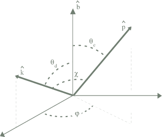
It is possible to take advantage of the azimuthal symmetry of the distribution function
around the field line direction as well as the relations between angles χ, θe and θd using
projection on Legendre polynomials, in order to reduce the required number of integrations. The
numerical accuracy for the determination of dnk∕dtdkdΩ may be then greatly enhanced,
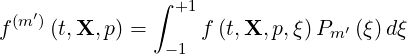
while the computational time strongly reduced. Let define the series for a function
h
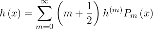 | (3.507) |
where coefficients h
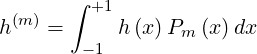 | (3.508) |
and Pm is the Legendre polynomial of degree m.
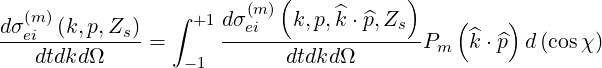
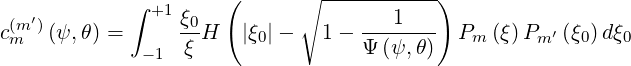
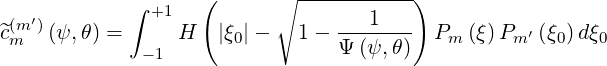
Applying the Legendre polynomial series to differential cross-sections dσei∕dtdkdΩ and
dσee∕dtdkdΩ and to f ,
,
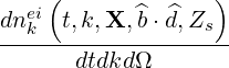 | = ns ∫
0∞vp2dp∫
02πdφ∫
-1+1dξ× ∫
0∞vp2dp∫
02πdφ∫
-1+1dξ× | ||
∑
m=0∞∑
m′=0∞   × × | |||
f  P
m P
m Pm′ Pm′ | (3.509) |
where
 | (3.510) |
and
 | (3.511) |
one obtains
 | = ns ∫
0∞vp2dp∑
m=0∞∑
m′=0∞ ∫
0∞vp2dp∑
m=0∞∑
m′=0∞  × × | ||
 f f  × × | |||
∫
02πdφ∫
-1+1dξP
m Pm′ Pm′ | (3.512) |
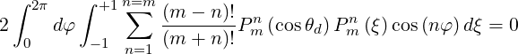
Using the well known sum relation for the Legendre polynomials that holds for angle relation between χ, θe and θd,
 | (3.513) |
where Pmn is the associated Legendre function of degree m and order n, expression (3.512)
becomes
is the associated Legendre function of degree m and order n, expression (3.512)
becomes
 | = ns ∫
0∞vp2dp∑
m=0∞∑
m′=0∞ ∫
0∞vp2dp∑
m=0∞∑
m′=0∞  × × | ||
 f f  ∫
02πdφ× ∫
02πdφ× | |||
∫
-1+1P
m Pm Pm Pm′ Pm′ dξ dξ | (3.514) |
since
 | (3.515) |
after permutation of integrals over ξ and φ. Using finally the orthogonality relation
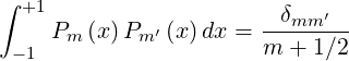 | (3.516) |
where δmm′ is the Kronecker symbol, one obtains the simple relation
 | = 2πns ∫
0∞vp2dp∑
m=0∞ ∫
0∞vp2dp∑
m=0∞ × × | ||
 f f  P
m P
m | (3.517) |
or
 = 2πns = 2πns ∑
m=0∞ ∑
m=0∞ × × | |||
Pm ∫
0∞vp2 ∫
0∞vp2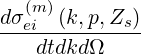 f f  dp dp | (3.518) |
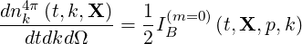
A similar expression may be obtained for the e-e bremsstrahlung, and the total bremsstrahlung is then
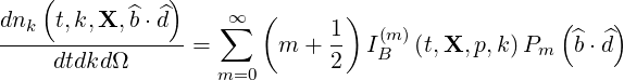 | (3.519) |
where the bremsstrahlung function IB
 is
is
IB  | = 2π ∫
0∞vp2f   dp dp | ||
![]
dσ(eme)(k,p)-
+ne (t,X) dtdkd Ω](NoticeDKE1676x.png) dp dp | (3.520) |
and the densitites ns = ns
= ns and ne
 = ne
= ne are considered to be uniform
on a magnetic flux surface ψ.
are considered to be uniform
on a magnetic flux surface ψ.
With this formulation, bremsstrahlung emission may be determined for any direction of
observation with the same numerical accuracy. Indeed, the projection of the distribution
function and the differential cross-sections over the Legendre polynomial basis is equivalent to
determine their value for all azimuthal directions. It is then only necessary to select the
interesting direction that is given by the local  ⋅
⋅ value, which depends of the local
instrumental arrangement, but also of the magnetic equilibrium. This formulation is particularly
convenient when the instrument is made of different chords with different orientations. It is not
only important for tangential observation of the plasma, but also for perpendicular ones, since
value, which depends of the local
instrumental arrangement, but also of the magnetic equilibrium. This formulation is particularly
convenient when the instrument is made of different chords with different orientations. It is not
only important for tangential observation of the plasma, but also for perpendicular ones, since
 ⋅
⋅ evolves with ψ as a consequence of the local magnetic shear. Moreover, this method offer the
advantage to evaluate dσei
evolves with ψ as a consequence of the local magnetic shear. Moreover, this method offer the
advantage to evaluate dσei
 ∕dtdkdΩ and dσee
 ∕dtdkdΩ only once for
various distribution functions, a procedure which may save considerably computer time
consumption when the distribution function and the plasma equilibrium, i.e.
∕dtdkdΩ only once for
various distribution functions, a procedure which may save considerably computer time
consumption when the distribution function and the plasma equilibrium, i.e.  ⋅
⋅ evolves with
the time t.
evolves with
the time t.
From expression (3.519), it is also possible to extract interesting local quantities about the
bremsstrahlung, like the mean radiation level in all directions of the configuration space
dnk4π ∕dtdkdΩ
 | =  ∫ ∫
 dΩ dΩ | ||
=  ∫
0πdθ
d ∫
-ππ sinθ
ddφd ∫
0πdθ
d ∫
-ππ sinθ
ddφd | (3.521) | ||
=  ∫
-11dξ
d ∫
-11dξ
d | (3.522) | ||
=  ∑
m=0∞ ∑
m=0∞ IB IB  ∫
-11dξ
dPm ∫
-11dξ
dPm | (3.523) |
and since P0 = 1, using the orthogonality relation (3.516), one obtains
 | (3.524) |
Much in the same way, the local anisotropy of the photon emission RB may be
evaluated from the ratio between the forward emission corresponding to cosθd = 1 and the
perpendicular one corresponding to cosθd = 0.
may be
evaluated from the ratio between the forward emission corresponding to cosθd = 1 and the
perpendicular one corresponding to cosθd = 0.
The determination of IB
 requires to evaluate the projection of the
electron distribution function given by the electron drift kinetic equation, at all X
positions.6
Since the magnetic configuration is a toroidaly symmetric, only the radial ψ and
poloidal θ positions are necessary, and therefore f
requires to evaluate the projection of the
electron distribution function given by the electron drift kinetic equation, at all X
positions.6
Since the magnetic configuration is a toroidaly symmetric, only the radial ψ and
poloidal θ positions are necessary, and therefore f = f
= f . Since
f
. Since
f
 is a linear function of f
 , it may be split into the three contributions,
namely
, it may be split into the three contributions,
namely
f  | = f
0  + f
1 + f
1  | ||
= f0  + +    + g + g  | (3.525) |
where f0
 are the Legendre coefficients for the zero order distribution
function f0, while f1
are the Legendre coefficients for the zero order distribution
function f0, while f1
 correspond to the first order distribution function
f1.
correspond to the first order distribution function
f1.
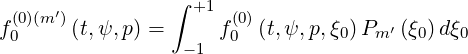
Like for other moments of the distribution function, starting from the angular relation
 | (3.526) |
and using the relation ξdξ = Ψ ξ0dξ0, one obtains for the zero order distribution function
f0
ξ0dξ0, one obtains for the zero order distribution function
f0
f0  | = ∫
-1+1f
0 Pm Pm dξ dξ | ||
= Ψ ∫
-1+1f
0 ∫
-1+1f
0   × × | |||
H Pm Pm dξ0 dξ0 | (3.527) |
since f0 is constant along a magnetic field line, i.e. f0 = f0
= f0
 . Here
the Heaviside function H indicates that only electrons who reach the poloidal position θ must be
considered. By expanding part of the integrand in (3.527) as a series of Legendre polynomials,
according to the relation
. Here
the Heaviside function H indicates that only electrons who reach the poloidal position θ must be
considered. By expanding part of the integrand in (3.527) as a series of Legendre polynomials,
according to the relation
 | (3.528) |
with
 | (3.529) |
one obtains finaly
 | (3.530) |
or
 | (3.531) |
where
 | (3.532) |
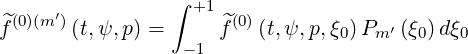
For the first order distribution function, f1 =  + g, since g is constant is constant along a
field line, its contribution is the same as for f0. Because
+ g, since g is constant is constant along a
field line, its contribution is the same as for f0. Because  has an explicit dependence upon θ,
which is given by relation (3.280),
has an explicit dependence upon θ,
which is given by relation (3.280),
   | = ∫
-1+1  P
m P
m dξ dξ | ||
= ∫
-1+1   H H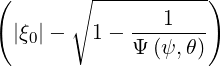 Pm Pm dξ0 dξ0 | |||
| (3.533) |
If
 | (3.534) |
with
 | (3.535) |
then expression (3.533) becomes
 | (3.536) |
Since
 | (3.537) |
one obtains finaly
 | (3.538) |
It is interesting to notice that the determination of the f
 does not require the
explicit evaluation of the distribution function f
does not require the
explicit evaluation of the distribution function f at all poloidal positions, and
only its value at Bmin is needed for the 4 - D problem that is represented by the
bremsstrahlung. This result which is a direct consequence of the weak collisional or “banana”
regime, is very important for the numerical evaluation. Indeed, all the physics of the
trapped-passing electrons is incorporated in the coefficients f
at all poloidal positions, and
only its value at Bmin is needed for the 4 - D problem that is represented by the
bremsstrahlung. This result which is a direct consequence of the weak collisional or “banana”
regime, is very important for the numerical evaluation. Indeed, all the physics of the
trapped-passing electrons is incorporated in the coefficients f
 , while the
contribution arising from magnetic field line helicity is independently described by
cosθd =
, while the
contribution arising from magnetic field line helicity is independently described by
cosθd =  ⋅
⋅ .
.