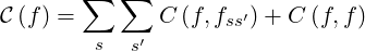
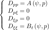
The collision operator used in the calculations may be expressed as1
|
| (4.1) |
where ∑
s ∑
s′C describe interactions between electrons and ions of species s in the
ionization state s′ and C
describe interactions between electrons and ions of species s in the
ionization state s′ and C is the self-collision contribution, as discussed in Ref. [?]. For the
electron-ion collisions, it is considered that fss′ is a Maxwellian distribution function, the
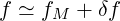
corresponding temperature being Tss′. In the application of the code here foreseen, including RF
heating and current drive, collisions dominate thermal particles, and therefore the
distribution function f may be expanded about the Maxwellian fM according to the
relation
is the self-collision contribution, as discussed in Ref. [?]. For the
electron-ion collisions, it is considered that fss′ is a Maxwellian distribution function, the
corresponding temperature being Tss′. In the application of the code here foreseen, including RF
heating and current drive, collisions dominate thermal particles, and therefore the
distribution function f may be expanded about the Maxwellian fM according to the
relation
 | (4.2) |
The self-collision operator C may be consequently approximated by its linearized
form
may be consequently approximated by its linearized
form
 | (4.3) |
where the the relation C = 0 has been used, and terms of order δf2 have been ignored.
It can be shown that the operator C
= 0 has been used, and terms of order δf2 have been ignored.
It can be shown that the operator C may be computed as C
 and expressed in a
conservative form
and expressed in a
conservative form
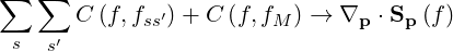 | (4.4) |
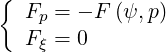
where component Sp and Sξ of the flux Sp are
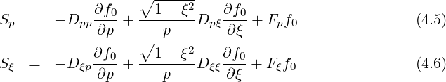
In the standard notations used in Ref. [?]
 | (4.7) |
and
 | (4.8) |
The term C requires is specific treatment. By expanding f as a sum of Legendre
harmonics according to the relation
requires is specific treatment. By expanding f as a sum of Legendre
harmonics according to the relation
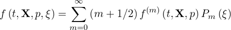 | (4.9) |
with
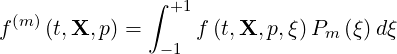 | (4.10) |
one obtains
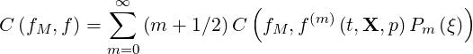 | (4.11) |
By definition, f
 ≃ fM and, since P0
 = 1,
= 1,

The first non-zero term in the series is then kept, so that
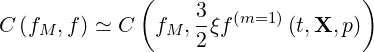 | (4.12) |
since P1 = ξ. By construction the linearized electron-electron collision operator conserves
momentum, but not energy, so there is no need to introduce an energy loss term in the kinetic
equation. Since f
= ξ. By construction the linearized electron-electron collision operator conserves
momentum, but not energy, so there is no need to introduce an energy loss term in the kinetic
equation. Since f is an integral of f, the term C
 introduce a non-linear dependence
in the Fokker-Planck or drift kinetic equation. However, even if it is crucial for the current drive
problem, including the determination of the boostrap current level, this non-linearity
remains weak, so that the rate of convergence towards the solution of the kinetic
equation is not significantly affected, even if this term is treated explicitely, regarding the
time scheme. For the calculations, the notation used in Ref. [?] is considered, and
introduce a non-linear dependence
in the Fokker-Planck or drift kinetic equation. However, even if it is crucial for the current drive
problem, including the determination of the boostrap current level, this non-linearity
remains weak, so that the rate of convergence towards the solution of the kinetic
equation is not significantly affected, even if this term is treated explicitely, regarding the
time scheme. For the calculations, the notation used in Ref. [?] is considered, and
In the code, it is possible to choose different collision models for simulations. Most of them have been implemented for benchmarking, the only realistic one being the Belaiev-Budker relativistic collision operator.
In the calculations, the Belaiev-Budker collision operator is used for weakly relativistic plasmas.
This operator ranges from non-relativistic to fully relativistic limits and is therefore very well
suited for studying the heating and current drive problems. Its recent formulation in terms of
Rosenbluth-like potential has open the possibility to use it in numerical calculations (Ref.[?]).
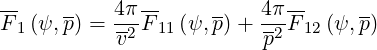
Following the work done in Ref. [?] , normalized coefficients Aee , Fee
, Fee and Btee
 are
are
 | (4.14) |
and
 | (4.15) |
Here,
 | (4.16) |
 | (4.17) |
 | (4.18) |
 | (4.19) |
 | (4.20) |
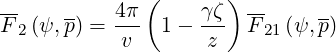
When relativistic corrections are neglected, 1 - γζ∕z ≈ 0, expressions derived from usual Rosenbluth potentials are recovered [?], and
 | (4.21) |
and
 | (4.22) |
with
 | (4.23) |
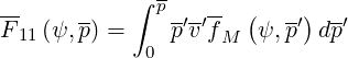
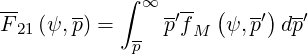
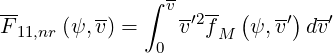
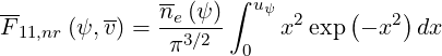
since p = v in this limit. The expression of F11,nr for a Maxwellian background is
![-- ∫ v ( -′2 )
F11,nr (ψ, v) = ---ne-(ψ-)---- v′2 exp - --v---- dv′
[2πTe (ψ )]3∕2 0 2Te(ψ )](NoticeDKE1818x.png) | (4.24) |
can then be evaluated analyticaly using the coordinate transformation uψ = v∕ ,
,
 | (4.25) |
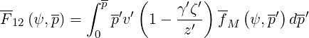
and by integrating by parts
![∫ uψ ( ) [ ( )]u ∫ uψ ( )
exp - x2 dx = x exp - x2 0ψ+ 2 x2 exp - x2 dx
0 0](NoticeDKE1821x.png) | (4.26) |
one obtains
![-- -- [ ]
F11,nr(ψ, v) = ne(ψ)-Erf (uψ)- u ψErf ′(u ψ)
4π](NoticeDKE1822x.png) | (4.27) |
where
 | (4.28) |
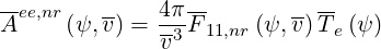
Consequently
![-- n- (ψ) [ ]
Fee,nr(ψ, v) =--e2-- Erf (u ψ)- uψErf ′(uψ )
v](NoticeDKE1824x.png) | (4.29) |
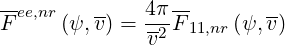
and for Aee,nr it comes
![-- --
Aee,nr(ψ,v-) = ne-(ψ)T-e(ψ) [Erf (u )- u Erf ′(u )]
v3 ψ ψ ψ](NoticeDKE1826x.png) | (4.30) |
expressions which correspond to the Maxwellian limit discussed later in this section.
The high velocity limit corresponds to the condition uψ ≫ 1, and in this case, since
limuψ→∞Erf = 1, it comes readily
 | (4.31) |
and
 | (4.32) |
which both are well known relations.
Much in the same way, the expression of coefficient Btee for pitch-angle scattering is
 | (4.33) |
with

n=1](NoticeDKE1831x.png) | (4.34) |
and
![-- -- ∑5 --[n] --
Bt2(ψ,p) = 4π B t2 (ψ, p)
n=1t2](NoticeDKE1832x.png) | (4.35) |
where
 = -1- p′2f-M (ψ,p′)dp′
t1 2v 0](NoticeDKE1833x.png) | (4.36) |
![-
--[2] -- 1 ∫ p-′4-- ( -′) -′
B t1 (ψ,p) = - 6vp2 p f M ψ,p dp
0](NoticeDKE1834x.png) | (4.37) |
![-- ∫ p -′ -- ( )
B[t31] (ψ, p) = --1--- p′2J1-(p-)fM ψ, p′ dp′
8γ2z2 0 γ′](NoticeDKE1835x.png) | (4.38) |
![∫ - --
--[4] -- --1---- p-′2 J2(p′)-- ( -′) -′
B t1 (ψ,p) = - 4z2 0 p γ′ f M ψ,p dp
i+1∕2](NoticeDKE1836x.png) | (4.39) |
![-
--[5] -- 1 ∫ pp′2( ′ ζ′) -- ( --′) -′
B t1 (ψ,p) = ----2--- γ-′ γ - z′ fM ψ,p dp
4γ i+1∕2 0](NoticeDKE1837x.png) | (4.40) |
and
 = 1- p--fM (ψ,p′)dp′
2 p v′](NoticeDKE1838x.png) | (4.41) |
![∫ --
--[2] -- γ2- ∞ -p′2--- -′
B t2 (ψ,p) = - 6 p γ′2v′fM dp](NoticeDKE1839x.png) | (4.42) |
![-[3] -- J1 (p)∫ ∞ p-′2 1 -- ( -′) -′
Bt2 (ψ, p) =-8γz2 - -v′γ-′2fM ψ, p dp
p](NoticeDKE1840x.png) | (4.43) |
 = - γJ2(2p)- p′-1′2-fM ψ,p′ dp′
4z p v γ](NoticeDKE1841x.png) | (4.44) |
 = ---1-- γ - ζ- p′2v′f- (ψ, p′) dp′
t2 4γ p2 z p M](NoticeDKE1842x.png) | (4.45) |
Here,
 | (4.46) |
 | (4.47) |
with
 | (4.48) |
 | (4.49) |
 | (4.50) |
and fM is the weakly relativistic normalized Maxwellian distribution function given in
Sec.6.3.5.
is the weakly relativistic normalized Maxwellian distribution function given in
Sec.6.3.5.
The first order Legendre correction of the collision operator 
 is expressed
as
is expressed
as
 | |||
=  f f  + +  1 1 + p2 + p2 | (4.51) |
where
![--(-- -(m=1) --) ∑10 -[n] --
I1 f M,,f0 (ψ,p) = I1 (ψ,p )
n=1](NoticeDKE1857x.png) | (4.52) |
and
![7
--(-- -(0)(m=1) --) ∑ -[n] --
I2 f M,,f0 (ψ,p) = I2 (ψ,p )
n=1](NoticeDKE1858x.png) | (4.53) |
The set of coefficients 1![[n]](NoticeDKE1859x.png)
 is
is
![-
-[1] -- 1 ∫ p p′3--(m=1 ) -- -′
I1 (ψ, p) = --------- γ′f 0 (ψ,p)dp
3Te,l+1∕2 0](NoticeDKE1861x.png) | (4.54) |
 = - ---i+1∕2-- p′3f(0m=1)(ψ, p)dp′
3Te,l+1∕2 0](NoticeDKE1862x.png) | (4.55) |
![∫ -
-[3] -- -γi+1∕2--- p p′5--(m=1 ) -- -′
I1 (ψ, p) = 5T2 0 γ′f 0 (ψ,p)dp
e,l+1∕2](NoticeDKE1863x.png) | (4.56) |
![-
-[4] -- ∫ p p′( ′ ζ′) -(m=1) -- -′
I1 (ψ,p) = γ′ γ - z′ f0 (ψ,p) dp
0](NoticeDKE1864x.png) | (4.57) |
 = - --i+1∕2- p--J2(p-)f(0m=1)(ψ,p) dp′
Te,l+1∕2 0 γ ′ z ′2](NoticeDKE1865x.png) | (4.58) |
![-- -- ∫ --- ( )
-[6] -- γp2 --5T-e(ψ) pp′3 3-- 3γ′ζ′ --(m=1 ) -- -′
I1 (ψ, p) = 6T-2(ψ) 0 γ′ 1+ z′2 - z′3 f 0 (ψ,p)dp
e](NoticeDKE1866x.png) | (4.59) |
![-
-[7] -- γ ∫ p p′3J3 (p′)--(m=1 ) -- -′
I1 (ψ, p) = --†2-2---- γ′--z-′-f 0 (ψ,p)dp
2βth Te (ψ ) 0](NoticeDKE1867x.png) | (4.60) |
 = ---γ--- p--J1(p-)f(m=1)(ψ,p) dp′
1 2T e(ψ) 0 γ ′ z′2 0](NoticeDKE1868x.png) | (4.61) |
![-- ∫ --- ( )
-[9] -- --p2-- pp′ γ-′ζ′ --(m=1 ) -- -′
I1 (ψ, p) = T-e(ψ) 0 γ ′ z′ - 1 f 0 (ψ,p)dp](NoticeDKE1869x.png) | (4.62) |
![-
-[10] -- γ2 ∫ pp′3J4 (ψ )-(m=1) -- -′
I1 (ψ,p) = -----†2-2--- -γ′--z′--f0 (ψ, p)dp
12 βthT e (ψ) 0](NoticeDKE1870x.png) | (4.63) |
and the coefficients 2![[n]](NoticeDKE1871x.png)
 are
are
 = ---1--- 1-f(0m=1)(ψ,p) dp′
3T e(ψ) p γ′](NoticeDKE1873x.png) | (4.64) |
![( ) ∫
--[2] -- --2γ--- --p2--- ∞ -(m=1 ) -- -′
I 2 (ψ,p) = - 3T- (ψ) + -2 - f0 (ψ, p)dp
e 5Te (ψ) p](NoticeDKE1874x.png) | (4.65) |
![( )
-[3] -- ζ 1 ∫ ∞ 1 -(m=1) -- -′
I2 (ψ,p) = γ - z- p2 - γ′f0 (ψ,p) dp
p](NoticeDKE1875x.png) | (4.66) |
![--[4] -- J (p) ∫ ∞ -(m=1) -- --
I 2 (ψ,p) = - -22----- - f0 (ψ, p)dp′
z Te(ψ) p](NoticeDKE1876x.png) | (4.67) |
 = 1+ 3-- 3γζ- ---1--- γ′p----5T-e(ψ)- f (m0=1 )(ψ,p)dp′
z2 z3 6T 2e (ψ) p γ′](NoticeDKE1877x.png) | (4.68) |
![( )
-[6] -- J3(p) J1(p) J4(p) ∫ ∞ -(m=1) --
I2 (ψ,p) = ---†2-2----+ --2------- -----†2-2--- - f0 (ψ,p) dp′
2zβthTe (ψ ) 2z Te(ψ ) 12z βth Te (ψ ) p](NoticeDKE1878x.png) | (4.69) |
 =----1--- γζ- 1 p- f-(m=1 )(ψ,p)dp′
2 p2T e(ψ) z p γ′ 0](NoticeDKE1879x.png) | (4.70) |
where
 | (4.71) |
 | (4.72) |
The relativistic Maxwellian limit corresponds to that case where the first order Legendre
correction for momentum conservation is neglected, but nevertheless using the Beliaev-Budker
formulation for coefficients Aee , Fee
, Fee and Btee
 . This is an academic case that
allows only fruitful comparison with some theorerical works for code benchmarking.
. This is an academic case that
allows only fruitful comparison with some theorerical works for code benchmarking.
The non-relativistic collision operator with a Maxwellian background is extensively discussed in Ref. [?]. It is an interesting model, since analytical evaluation of the collision integrals may be performed. Its validity is restricted to the limit γ - 1 ≪ 1, where γ is the Lorentz factor defined is Sec.6.3.4. In that case v = p is the unit system here employed. Using the standard notations
![--
--ee -- ne(ψ-)-1-[ ′ ]
A (ψ,p) = 2v- u2ψ Erf (uψ)- uψErf (uψ)](NoticeDKE1885x.png) | (4.73) |
![-ee -- ne (ψ)[ ′ ]
F (ψ,p ) =--v2-- Erf (u ψ)- uψErf (uψ )](NoticeDKE1886x.png) | (4.74) |
and
![-ee -- ne (ψ) 1 [( ) ]
Bt (ψ,p) = -------2- 2u2ψ - 1 Erf (u ψ)+ uψErf ′(uψ )
4v uψ](NoticeDKE1887x.png) | (4.75) |
where
 | (4.76) |
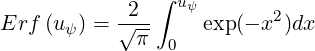
 | (4.77) |
is the well know error function defined in Refs [?] and [?] , and its derivative
 | (4.78) |
The relation
 | (4.79) |
which ensures that the Maxwellian is the correct solution when collisions is the only physical process. In that limit, self-collisions are neglected.
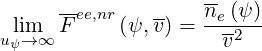
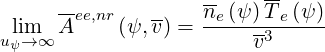
Though the high velocity limit uψ ≫ 1 corresponds to a restricted range of applications regarding the full electron-electron collision operator, it can contribute usefuly to comparisons with some theoretical calculations. Starting from expressions given in Ref. [?],
 | (4.80) |
 | (4.81) |
and
![-ee -- ne (ψ)[ T-e(ψ)]
Bt (ψ,p) = ------ 1 - ---2--
2v v](NoticeDKE1894x.png) | (4.82) |
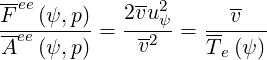
With these definitions, the ratio
 | (4.83) |
is well recovered. In that limit, self-collisions are neglected.
This case corresponds to the limit where only pitch-angle scattering of electrons on massive ions
with Tss′ = 0, with large Zss′. Consequently, large simplifications may be performed,
and
= 0, with large Zss′. Consequently, large simplifications may be performed,
and
 | (4.84) |
This simple model is very interesting since analytical expressions may be obtained in this limit, which allow accurate code benchmarking, especially for the bootstrap current problem in arbitrary magnetic configuration. Obviously, self-collisions are neglected by definition.
The growth rate of runaway electrons by a large constant electric field is often studied using the
ultra-relativistic model as derived by C. Møller in the early 1930’s [?]. In this limit, since the
ratio of the friction term Fee to the diffusion one Aee
 scales like v as indicated in 4.79
, the contribution of the diffusion Aee
scales like v as indicated in 4.79
, the contribution of the diffusion Aee is simply neglected in the limit v → c.
Hence,
is simply neglected in the limit v → c.
Hence,
 | (4.85) |
and
 | (4.86) |
For the pitch-angle term, the term is simply
 | (4.87) |
It is important to recall that the term βth† arises from the definition of the normalization for
p as discussed in Sec.6.3.4. It can be observed that the Møller collision model is equivalent for
e-e interactions to the high-velocity limit of the e-e standard collision operator, neglecting all
terms of the order of v-3. Therefore, the model may have analytical solutions since
the partial derivative in p of the collision operator is of the first order. However, as
-vAee ∕Fee
∕Fee ≠Te
≠Te high numerical instabilities are found in the code. This model is
equivalent to Te
high numerical instabilities are found in the code. This model is
equivalent to Te = 0 which is obviously not consistent with the initial assumptions.
Therefore, in order to ensure a correct numerical stability, the expression 4.80 for Aee
= 0 which is obviously not consistent with the initial assumptions.
Therefore, in order to ensure a correct numerical stability, the expression 4.80 for Aee is
used with the Møller model. It has been cross-checked that this does not change the final
results.
is
used with the Møller model. It has been cross-checked that this does not change the final
results.
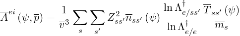
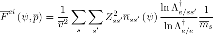
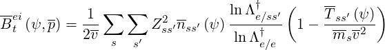
Since ions mass is much larger than electron ones, their dynamics is almost non-relativistic. Consequently, electron-ion collisions may be described in this limit considering a Maxwellian ion background. Expressions for arbirary type of ions is also given in Ref. [?] and their validities are also restricted to the limit γ - 1 ≪ 1, where γ is the Lorentz factor defined is Sec.6.3.4. . In that case v = p is the unit system here employed. Using the standard notations
![-- ∑ ∑ [ ( ) ( )] ln Λ†
Aei(ψ,p) = -1- -1′--Erf usψs′ - uψErf ′ ussψ′ ---e∕ss′Z2ss′nss′ (ψ)
2v s s′ usψs2 lnΛ †e∕e](NoticeDKE1909x.png) | (4.88) |
![-- 1 ∑ ∑ [ ( ′) ′ ( ′)] ln Λ† ′ 1
F ei(ψ, p) =--2 Erf usψs - usψs Erf ′ usψs ---e∕†ssZ2ss′nss′ (ψ )--
v s s′ lnΛ e∕e ms](NoticeDKE1910x.png) | (4.89) |
and
![--ei -- 1 ∑ ∑ 1 [( ′ ) ( ′) ′ ( ′) ] lnΛ †e∕ss′ --
B t (ψ,p) =--- -ss′2- 2usψs2- 1 Erf usψs + usψsErf ′ usψs ----†---Z2ss′nss′ (ψ)
4v s s′ uψ ln Λe∕e](NoticeDKE1911x.png) | (4.90) |
where
 | (4.91) |
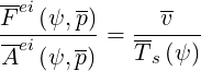
Here, vth,ss′† is the thermal velocity of species s in ionization state s′, while Erf(x) and Erf′(x) have the same expressions as for the electron-electron collision term. For a single ion species s fully ionized, the ratio
 | (4.92) |
which means that the electron population is thermalized to the ion temperature Ts . The
quantities lnΛe∕ss′† and lnΛe∕e† are the reference Coulomb logarithms defined in Sec.
6.3.4.
. The
quantities lnΛe∕ss′† and lnΛe∕e† are the reference Coulomb logarithms defined in Sec.
6.3.4.
For most current drive studies like for the Lower Hybrid wave where the resonance condition is
far from the thermal bulk, it is reasonable to consider the high velocity limit of the
electron-ion collision operator. Corresponding coefficients Aei , Fei
, Fei and Btei
 are
are
 | (4.93) |
 | (4.94) |
and
 | (4.95) |
where the double sum ∑
s ∑
s′ takes into account of all ions species s in ionization state s′.
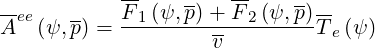
Here, nss′ is the normalized ion density at ψ, as introduced in Sec. 6.3.1, and
ms is the ion rest mass normalized to the electron rest mass me. Coefficients for the
electron-ion collisions given in Ref.[?] are well recovered. Like for the Maxwellian
limit,
is the normalized ion density at ψ, as introduced in Sec. 6.3.1, and
ms is the ion rest mass normalized to the electron rest mass me. Coefficients for the
electron-ion collisions given in Ref.[?] are well recovered. Like for the Maxwellian
limit,
 | (4.96) |
which means that the electron population is thermalized to the ion temperature Ts , when a
single ion species s is considered.
, when a
single ion species s is considered.
Since only pitch-angle electron scattering on massive ions with Tss′ = 0, with large Zss′ is
considered in this model, by definition
= 0, with large Zss′ is
considered in this model, by definition
 | (4.97) |
while
 | (4.98) |
The solutions of the Fokker-Planck and the drift kinetic equations is independent in this limit of the Btei value. Here the standard value 1∕2 is chosen as used in several publications for analytical calculations.
A simplified term is used where
 | (4.99) |
since ion contribution is almost negligible as compared to electrons and
 | (4.100) |
by combining the high-velocity limit expression 4.95, and the momentum dependence given in Ref. [?].
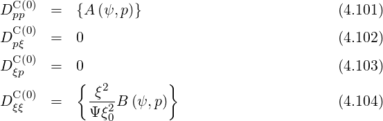
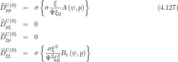
In the Fokker-Planck equation, the diffusion and convection elements are bounce-averaged according to the expressions (3.189)-(3.194), which gives, using (4.7)-(4.8),
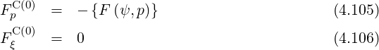
Here, coefficients A
 , Bt
, Bt
 and F
and F
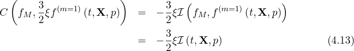
 are determined at the location where
B = B0 on the magnetic flux surface. However, since A, Bt and F are only functions of
the density and temperature that are flux surface quantities as shown in Sec. 4.1.1,
their respective values are consequently independent of the poloidal position and
therefore, A
are determined at the location where
B = B0 on the magnetic flux surface. However, since A, Bt and F are only functions of
the density and temperature that are flux surface quantities as shown in Sec. 4.1.1,
their respective values are consequently independent of the poloidal position and
therefore, A = A, Bt
 = Bt and F
 = F. The bounce coefficient λ2,-1,0 is defined as
(2.66)
= F. The bounce coefficient λ2,-1,0 is defined as
(2.66)
 | (4.113) |
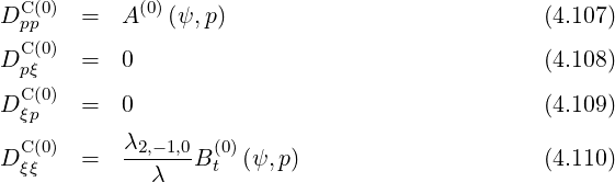
For reference to the litterature ([?]), note that we could also perform the following transformation
 | (4.115) |
The evaluation of Δb for circular concentric flux surfaces in given in Appendix ??.
Concerning the term that ensures momentum conservation in the collision operator, one must evaluate
 | (4.116) |
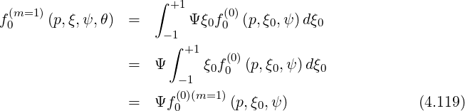
Making the substitution Ψξ0dξ0 = ξdξ in the integral f0 = ∫
-1+1ξf0
= ∫
-1+1ξf0 dξ, one
obtains
dξ, one
obtains
 | (4.117) |
where the limits of integration come from the relation ξ = σ
= σ .
Since f0
.
Since f0 is symmetric in the region of the phase space ξ0 ∈
 which
corresponds to trapped orbits,
which
corresponds to trapped orbits,
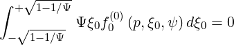 | (4.118) |
one get


 is the Legendre integral evaluated at B0 = B
 , independent of θ.
Since the operator is linear,
, independent of θ.
Since the operator is linear, 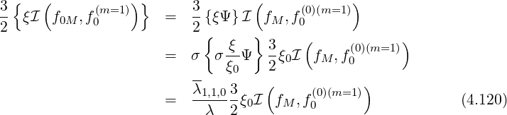
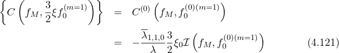
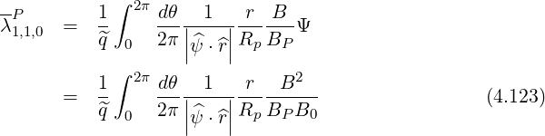
Expression of λ1,1,0 This coefficient is expressed as
![[ ]
-- σ 1 ∑ ∫ θmax dθ 1 r B
λ1,1,0 = -- -- ---||---||------ σΨ
^q 2 σ T θmin 2π |ψ^⋅^r| RpBP](NoticeDKE1961x.png) | (4.122) |
Since the integral is odd in σ, the sum over trapped particles vanishes, λ1,1,0 = 0 for trapped electrons, and λ1,1,0 = λ1,1,0P ≠0 for circulating ones. Hence
Case of circular concentric flux-surfaces
In this case, ϵ = r∕Rp,  ⋅
⋅ = 1 and since the ratio B∕BP is a function of r only
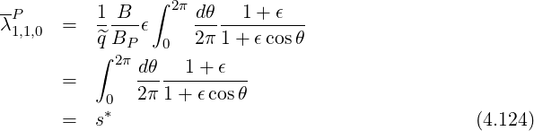
 BP ∕B = ϵ. The integral s*, according to the old notations found in the
litterature ([?]),
BP ∕B = ϵ. The integral s*, according to the old notations found in the
litterature ([?]),
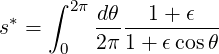 | (4.125) |
can be performed analytically, as shown in Appendix ??, and
 | (4.126) |
Moreover, in this limit, λ1,1,0P = λ1,-1,2P , as shown in Sec.4.2.2.
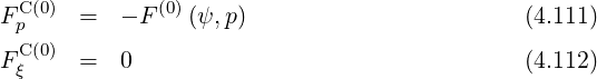
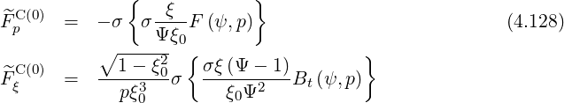
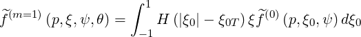
In the first order drift kinetic equation, the diffusion and convection flux elements related to  are bounce-averaged according to the expressions (3.218)-(3.223), which gives, using (4.7)-(4.8),
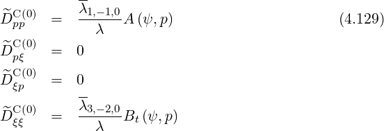
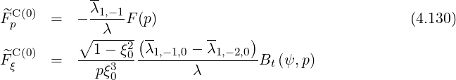
The following bounce coefficients are defined (2.66)
We also have the following relation, by expanding ξ2
 | (4.134) |
Concerning the term that ensures momentum conservation in the collision operator, one must evaluate
 | (4.135) |
Making like for the Fokker-Planck term the substitution Ψξ0dξ0 = ξdξ in the integral

 = ∫
-1+1ξ
= ∫
-1+1ξ
 dξ, one obtains
   | = | ∫
-1- Ψξ
0 Ψξ
0    dξ0 dξ0 | ||||
+ ∫
 +1Ψξ
0 +1Ψξ
0    dξ0 dξ0 | (4.136) |
which becomes
 | (4.137) |
Then,
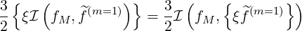 | (4.138) |
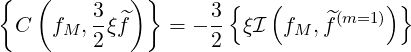
since fM and are independent of θ. It is therefore necessary to evaluate
![{ } 1 [ 1∑ ] ∫ θmaxdθ 1 r B ξ
ξf^(m=1 ) = --- -- ---|----|-------0ξf^(m=1)
λ ^q 2 σ T θmin 2π ||^ψ ⋅^r||Rp BP ξ
[ ] ∫
-1- 1∑ θmaxdθ-|-1--|r--B-- ^(m=1)
= λ ^q 2 θmin 2π |^ψ ⋅^r|Rp BP ξ0f
σ T | |
ξ0 ∫ 2π dθ 1 r B (m=1)
= λ-^qH (|ξ0|- ξ0T) 2π-||---||-R--B--^f (4.139)
0 |ψ^⋅^r| p P](NoticeDKE1996x.png)

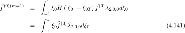
 is independent of σ because of the integration over ξ0, while
 ![[1∑ ]
2 σ](NoticeDKE1999x.png) T ξ0 = 0 for
trapped orbits. Hence,
T ξ0 = 0 for
trapped orbits. Hence, ![{ }
ξ^f(m=1)
∫ [ ∫ ]
ξ0- 2π dθ|--1-|-r--B- 3- 1 ^(0)
= λ^qH (|ξ0|- ξ0T) 0 2π|^ |Rp BP 2 -1H (|ξ0|- ξ0T)ξf dξ0
|ψ ⋅^r| ⌊ ⌋
∫ 1 ∫ 2π
= ξ0H (|ξ0|- ξ0T) H (|ξ0|- ξ0T) ^f(0)d ξ0 ⌈1 -dθ|-1--|-r--B-ξ⌉
λ -1 ^q 0 2 π||^ψ ⋅^r||Rp BP
⌊ ⌋
ξ ∫ 1 1 ∫ 2π dθ 1 r B ξ ξ2
= -0H (|ξ0|- ξ0T) H (|ξ0|- ξ0T) ^f(0)ξ0λd ξ0 ⌈-- --||----||------ -0-2⌉
λ -1 λ ^q 0 2π|ψ^⋅^r|Rp BP ξ ξ0
∫ 1 { 2}
= ξ0H (|ξ0|- ξ0T) ξ0H (|ξ0|- ξ0T ) ^f(0)λ ξ- dξ0
λ -1 ξ20
ξ0 ∫ 1
= --H (|ξ0|- ξ0T) ξ0H (|ξ0|- ξ0T ) ^f(0)λ2,0,0dξ0 (4.140)
λ -1](NoticeDKE2000x.png)
Defining
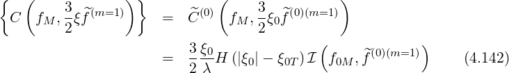
Note that in the case of circular concentric flux-surfaces, we can find analytical expressions for the bounce coefficients
 | (4.145) |
Furthermore,
![-- ∫ 2π dθ ξ
λ2,0,0 = H (|ξ0|- ξ0T) 2π-ξ-
∫02π 0 2
= H (|ξ0|- ξ0T) dθ-ξ0ξ-
0 2π ξ ξ20
∫ 2π dθ ξ 1- Ψ (1 - ξ2)
= H (|ξ0|- ξ0T) ----0------2----0-
0 2π ξ ξ0
-λ [ ( 2) ]
= H (|ξ0|- ξ0T)ξ20 1- 1 - ξ0 {Ψ } (4.146)](NoticeDKE2006x.png)
 given in Appendix ??,
 | (4.147) |
where J2m is expressed in terms of complete elliptic integrals of the first and second kind, and
 m is given by the recurrence relation
  m =
m = 
 m-1 with
  0 = 1,
![∞
-- 2- ∑ [ ( 2)] ξ20Tm-
λ2,0,0 = πH (|ξ0|- ξ0T) χm - ^χm 1- ξ0 ξ20 J2m
m=0](NoticeDKE2014x.png) | (4.148) |
Here χm is defined in Appendix ??. The series expansion is converging less rapidly than for λ0,0,0 = λ, therefore, at least first three terms have to be kept for accurate calculations, so that the truncated expression is
![-- [ ( ) ( ) ]
λ2,0,0 ≃ 2-H (|ξ0|- ξ0T) J0 + 1- 1- ξ20T J2 + 3-- -1- ξ40TJ4
π 2 ξ20 8 2ξ20](NoticeDKE2015x.png) | (4.149) |