
The coordinates  are defined on the space
| 0 ≤ R | < ∞ | ||
| -∞≤ Z | < ∞ | ||
| 0 ≤ ϕ | < 2π | (A.60) |
and is related to  by
by
| R | =  | (A.61) | |
| Z | = -z | ||
| ϕ | = arctan + πH + πH ![[2π]](NoticeDKE4453x.png) |
which is inverted to
| x | = R cosϕ | (A.62) | |
| y | = R sinϕ | ||
| z | = -Z |
The position vector then becomes
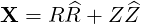 | (A.63) |
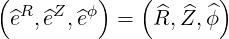
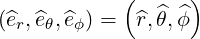
where we define a local orthonormal basis  as
as
 | = cosϕ + sinϕ + sinϕ | (A.64) |
 | = - | (A.65) |
 | =  × × = -sinϕ = -sinϕ + cosϕ + cosϕ | (A.66) |
The covariant vector basis is defined in (A.1), which becomes here
| eR | =  = =  | (A.67) |
| eZ | =  = =  | (A.68) |
| eϕ | =  = R = R = R = R | (A.69) |
so that we have the covariant basis
 | (A.70) |
the scaling factors
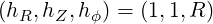 | (A.71) |
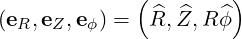
and the normalized tangent basis
 | (A.72) |
The Contravariant vector basis is defined in (A.9), which becomes here
| eR | = ∇R =  | (A.73) |
| eZ | = ∇Z =  | (A.74) |
| eϕ | = ∇ϕ =  | (A.75) |
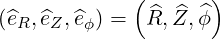
The relations (A.10-A.11) are here readily verified. The normalized reciprocal basis is
 | (A.76) |
which here coincides with the normalized tangent basis, since both bases are orthogonal.
They are defined in (A.12) and become here
| gij | = 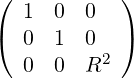 | (A.77) | |
| gij | = 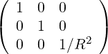 |
As a result
 | (A.78) |
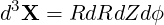
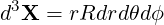
and the Jacobian is
 | (A.79) |
dl | = dR | (A.80) |
dl | = dZ | (A.81) |
dl | = Rdϕ | (A.82) |
dS | = RdZdϕ | (A.83) |
dS | = RdRdϕ | (A.84) |
dS | = dRdZ | (A.85) |
 | (A.86) |
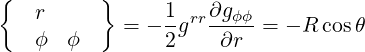
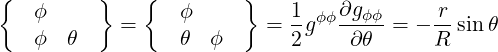
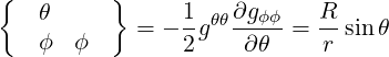
They are defined in (A.49) and are all zero here except
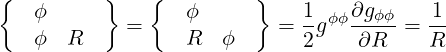 |
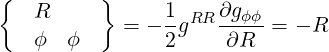 | (A.87) |
 | (A.88) |
 | (A.89) |
 ⋅ ⋅ | =   - -   | (A.90) |
 ⋅ ⋅ | =    - -   | (A.91) |
 ⋅ ⋅ | =   - -  | (A.92) |

The coordinates  are defined from the origin
  on the space
| 0 ≤ r | < ∞ | (A.93) | |
| 0 ≤ θ | < 2π |
and is related to  by
by
| r | = 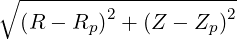 | (A.94) | |
| θ | = arctan + πH + πH ![[2π]](NoticeDKE4526x.png) |
which is inverted to
| R | = Rp + r cosθ | (A.95) |
| Z | = Zp + r sinθ | (A.96) |
The position vector then becomes
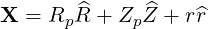 | (A.97) |
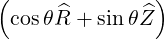
where we define a local orthonormal basis  as
as
 | = cosθ + sinθ + sinθ | (A.98) |
 | =  × × = -sinθ = -sinθ + cosθ + cosθ | (A.99) |
since
 × × | =  × × | (A.100) |
= ![[( ) ]
cosθR^+ sinθZ^ ⋅ ^R](NoticeDKE4541x.png)  - -![[( ) ]
cosθR^+ sinθ ^Z ⋅ ^Z](NoticeDKE4543x.png)  | (A.101) | |
= cosθ - sinθ - sinθ | (A.102) |
The covariant vector basis is defined in (A.1), which becomes here
| er | =  = =  | (A.103) |
| eθ | =  = r = r = r = r | (A.104) |
| eϕ | =  = Rp = Rp + r + r = =   = R = R | (A.105) |
so that we have the covariant basis
 | (A.106) |
the scaling factors
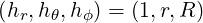 | (A.107) |
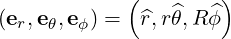
and the normalized tangent basis
 | (A.108) |
The Contravariant vector basis is defined in (A.9), which becomes here
| er | = ∇r =  | (A.109) |
| eθ | = ∇θ =   | (A.110) |
| eϕ | = ∇ϕ =  | (A.111) |
The relations (A.10-A.11) are here readily verified. The normalized reciprocal basis is
 | (A.112) |
which here coincides with the normalized tangent basis, since both bases are orthogonal.
They are defined in (A.12) and become here
| gij | = 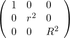 | (A.113) | |
| gij | = 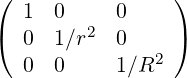 |
As a result
 | (A.114) |
and the Jacobian is
 | (A.115) |
dl | = dr | (A.116) |
dl | = dθ | (A.117) |
dl | = Rdϕ | (A.118) |
dS | = rRdθdϕ | (A.119) |
dS | = Rdrdϕ | (A.120) |
dS | = rdrdθ | (A.121) |
 | (A.122) |
They are defined in (A.49) and are all zero here except
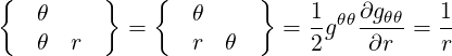 | (A.123) |
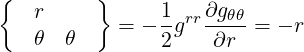 | (A.124) |
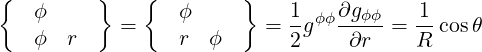 | (A.125) |
 | (A.126) |
 | (A.127) |
 | (A.128) |
 | (A.129) |
 | (A.130) |
 ⋅ ⋅ | =    - -   | (A.131) |
 ⋅ ⋅ | =    - -   | (A.132) |
 ⋅ ⋅ | =    - -   | (A.133) |

The coordinates  , used to parametrize closed flux-surfaces, are defined from the origin
 on the (closed) space
min | ≤ ψ ≤ max | (A.134) |
| 0 ≤ s ≤ smax | (A.135) |
and is related to  by
by
| ψ | = ψ | (A.136) | |
| s | = s |
which is inverted to
| r | = r | ||
| θ | = θ |
Note that ψ must be a monotonic function of r from ψ0 at the center
  to ψa at
the edge. It is the case for nested flux-surfaces.
to ψa at
the edge. It is the case for nested flux-surfaces.
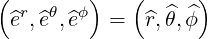
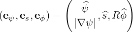
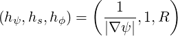
We define a local orthonormal basis  as
as
 | =  | (A.137) | |
 | =  × × |
The transformation from  to
to  is a rotation of angle α such that
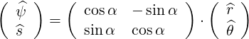 | (A.138) |
The position vector remains
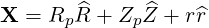 | (A.139) |
The covariant vector basis is defined in (A.1), which becomes here
| eψ | =  = =  s s + r + r s = s =  s s + r + r s s | (A.140) |
| es | =  = =  ψ ψ + r + r ψ = ψ =  ψ ψ + r + r ψ ψ | (A.141) |
| eϕ | =  = Rp = Rp + r + r = =   = R = R | (A.142) |
so that we have the covariant basis
 | (A.143) |
the scaling factors
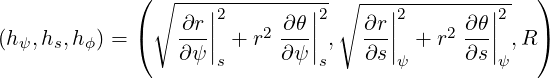 | (A.144) |
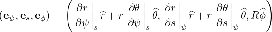
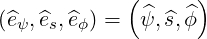
and the normalized tangent basis
![( | | [ | | ] )
1 [ ∂r | ∂θ | ] 1 ∂r| ∂θ|
(^eψ,^es,^eϕ) = h-- ∂ψ-|| ^r + r ∂ψ-|| ^θ ,h- ∂s|| ^r + r ∂s|| θ^ , ^ϕ
ψ s s s ψ ψ](NoticeDKE4658x.png) | (A.145) |
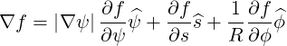
The Contravariant vector basis is defined in (A.9), which becomes here
| eψ | = ∇ψ =   | (A.146) |
| es | = ∇s =  | (A.147) |
| eϕ | = ∇ϕ =  | (A.148) |
The relations (A.11) then give
| eψ | =  = =  | (A.149) | |
| es | =  = =  | ||
| eϕ | =  = R = R |
so that we have the following tangent basis
 | (A.150) |
the scaling factors
 | (A.151) |
the normalized tangent basis
 | (A.152) |
the reciprocal basis
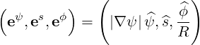 | (A.153) |
and the normalized reciprocal basis
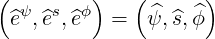 | (A.154) |
which here coincides with the normalized tangent basis, since both bases are orthogonal.
By comparing (A.143) with (A.149), we also find that
 s s | =  | (A.155) |
 s s | =  | (A.156) |
 ψ ψ | =  = sinα = sinα | (A.157) |
 ψ ψ | =  = =  | (A.158) |
They are defined in (A.12) and become here
| gij | = 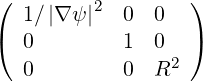 | (A.159) | |
| gij | = 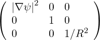 |
As a result
 | (A.160) |
and the Jacobian is
 | (A.161) |
dl | =  | (A.162) |
dl | = ds | (A.163) |
dl | = Rdϕ | (A.164) |
dS | = Rdsdϕ | (A.165) |
dS | =  dψdϕ dψdϕ | (A.166) |
dS | =  dψds dψds | (A.167) |
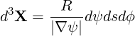 | (A.168) |
They are defined in (A.49) and are here
 | (A.169) |
 | (A.170) |
 ⋅ ⋅ | =    - -   | (A.171) | |
 ⋅ ⋅ | =    - -   | ||
 ⋅ ⋅ | =    - -   |

The coordinates  are defined from the origin
  on the space
 |
and is related to  by
by
 |
which is inverted to
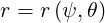 |
Note that ψ must be a monotonic function of r from ψ0 at the center
  to ψa at
the edge. It is the case for nested flux-surfaces.
to ψa at
the edge. It is the case for nested flux-surfaces.
The position vector then becomes
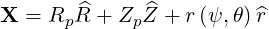 | (A.172) |
The covariant vector basis is defined in (A.1), which becomes here
| eψ | =  = =  θ θ | (A.173) |
| eθ | =  = =  ψ ψ + r + r = =  ψ ψ + r + r | (A.174) |
| eϕ | =  = Rp = Rp + r + r = =   = R = R | (A.175) |
so that we have the covariant basis
 | (A.176) |
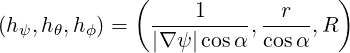
the scaling factors
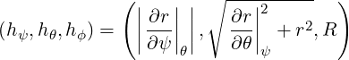 | (A.177) |
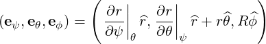
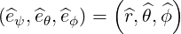
and the normalized tangent basis
![( [ | ] )
(^eψ,^eθ,^eϕ) = ^r, 1-- ∂r|| ^r + r^θ , ^ϕ
hθ ∂θ|ψ](NoticeDKE4754x.png) | (A.178) |
The Contravariant vector basis is defined in (A.9), which becomes here
| eψ | = ∇ψ =   | (A.179) |
| eθ | = ∇θ =  | (A.180) |
| eϕ | = ∇ϕ =  | (A.181) |
The relations (A.11) then give
| eψ | =  = =  | (A.182) |
| eθ | =  = =  = =  | (A.183) |
| eϕ | =  = R = R | (A.184) |
since  =
=  ×
× , so that we have the following tangent basis
 | (A.185) |
the scaling factors
 | (A.186) |
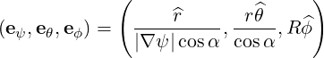
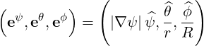
the normalized tangent basis
 | (A.187) |
the reciprocal basis
 | (A.188) |
and the normalized reciprocal basis
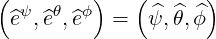 | (A.189) |
which here does not coincide with the normalized tangent basis, since both bases are not orthogonal.
By comparing (A.176) with (A.185), we also find that
 θ θ | =  | (A.190) |
 ψ ψ | = r = r tanα = r tanα | (A.191) |
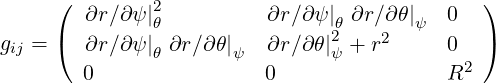
They are defined in (A.12) and become here
![( )
1∕ [|∇ψ |cosα]2 rtan α∕[|∇ ψ |cos α] 0
gij = ( rtan α∕ [|∇ψ |cosα] r2∕cos2α 0 )
0 0 R2](NoticeDKE4778x.png) | (A.192) |
or equivalently
 |
and
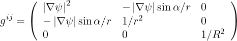 | (A.193) |
As a result
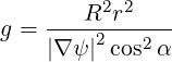 | (A.194) |
and the Jacobian is
 | (A.195) |
dl | =  | (A.196) |
dl | =  dθ dθ | (A.197) |
dl | = Rdϕ | (A.198) |
dS | =  dθdϕ dθdϕ | (A.199) |
dS | =  dψdϕ dψdϕ | (A.200) |
dS | =  dψdθ dψdθ | (A.201) |
 | (A.202) |
They are defined in (A.49) and are here
 | (A.203) |
 | (A.204) |
 ⋅ ⋅ | =    - -   | (A.205) |
 ⋅ ⋅ | =    - -   | (A.206) |
 ⋅ ⋅ | =    - -   | (A.207) |