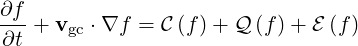
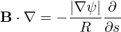
As shown in previous section, for axisymmetric plasmas, the electron drift kinetic equation may be expressed in the general form
|
| (3.31) |
where f = f is the guiding-center distribution function.
In tokamaks, it can be shown that the guiding center velocity vgc may be decomposed into a fast parallel motion along the field lines, and a vertical drift velocity vD across the magnetic flux surfaces
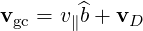 | (3.32) |
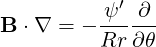
From the general expression (2.36) of the magnetic field B,
 | (3.33) |
one obtains in the  coordinates system,
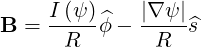 | (3.34) |
As shown in Appendix A, the gradient in  coordinates is
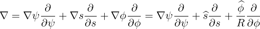 | (3.35) |
and recalling that the constants of the motion are the total energy (or momentum p) as defined in (2.16) and the magnetic moment μ as given by relation (2.17), following conservations laws
 | (3.36) |
![∂ [ 2 ]
---p ∥ + 2μBme = 0
∂s](NoticeDKE252x.png) | (3.37) |
are satisfied.
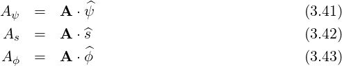
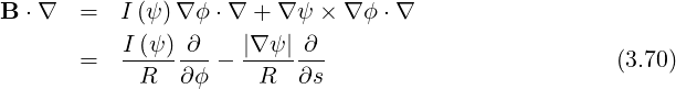
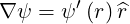
The toroidal canonical momentum is also a constant of the motion because of axisymmetry. It is expressed as
![Pϕ = R [γmevϕ + qeAϕ]](NoticeDKE253x.png) | (3.38) |
where Aϕ is the toroidal component of the vector potential. From the relation
 | (3.39) |
and the expression (A.171) of a rotational in  coordinates, we get
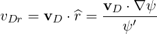
![[ ]
B = -1-∂-(RA ) - 1-∂--(A ) ψ^
R ∂s ϕ R ∂ϕ s
[ 1 ∂ |∇ ψ| ∂ ]
+ -----(A ψ)- ------- (RA ϕ) ^s
[R ∂ ϕ R ∂ ψ ( )]
+ |∇ψ |-∂-(A ) - |∇ ψ | ∂- -A-ψ- ^ϕ (3.40)
∂ψ s ∂s |∇ ψ|](NoticeDKE256x.png)
In axisymmetric plasma, this reduces to
so that
 | (3.45) |
In addition, we know from expression (3.34) that
 | (3.46) |
so that be obtain
 | (3.47) |
Because the toroidal canonical momentum is a constant of the motion, we have
 | (3.48) |
which can be decomposed into
 | (3.49) |
Using relation (A.169), we get
![[ ^ ]
vgc ⋅∇ (qeRA ϕ) = vgc ⋅ ∇ ψ ∂-+ ^s-∂-+-ϕ-∂- (qeRA ϕ )
∂ψ ∂s R ∂ ϕ](NoticeDKE264x.png) | (3.50) |
which in axisymmetric systems gives
![[ ]
v ⋅∇ (qA ) = qv ⋅ ∇ ψ∂RA--ϕ+ ^s∂RA-ϕ-
gc e ϕ e gc ∂ψ ∂s](NoticeDKE265x.png) | (3.51) |
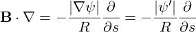
Since Bψ = 0, we have from relation (3.44) ∂ ∕∂s = 0 and therefore, using expression
(3.47),
∕∂s = 0 and therefore, using expression
(3.47),
 | (3.52) |
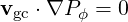
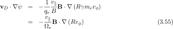
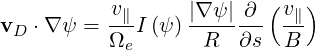
The only velocity accross the flux-surfaces is the drift velocity we are looking for, so that we get, using relation (3.32)
 | (3.53) |
and the equation (3.49) becomes
 | (3.54) |
Assuming a priori that  ≫
≫ , a condition that holds in tokamaks, this equation
reduces to
, a condition that holds in tokamaks, this equation
reduces to
The toroidal velocity is related to the parallel velocity by
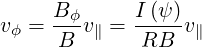 | (3.56) |
so that
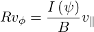 | (3.57) |
Since I is a flux function, it can be taken out of the gradient, so that
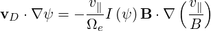 | (3.58) |
The guiding-center drift velocity due to the magnetic field gradient and curvature is
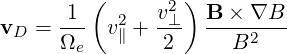 | (3.59) |
and its component perpendicular to the flux-surface can be written as
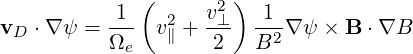 | (3.60) |
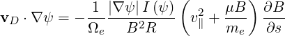
Inserting the expression (3.34) of the magnetic field, we find
![1 ( v2) |∇ ψ|[ ]
vD ⋅∇ψ = ---- v2∥ + -⊥- --2-- I (ψ)^s + |∇ ψ|ϕ^ ⋅∇B
Ωe 2 B R](NoticeDKE279x.png) | (3.61) |
Using (3.35), the equation (3.61) becomes
![( 2) [ ]
vD ⋅∇ψ = - 1-- v2+ v⊥- |∇-ψ| I (ψ) ∂B-+ |∇-ψ|∂B-
Ωe ∥ 2 B2R ∂s R ∂ ϕ](NoticeDKE280x.png) | (3.62) |
Under the assumption of axisymmetry, we are left with
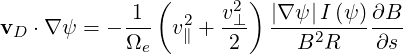 | (3.63) |
With the definition (2.17) of the magnetic moment μ, we rewrite
 | (3.64) |
We have, using the conservation of magnetic momentum (3.36),
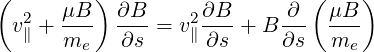 | (3.65) |
Using the conservation of energy (3.37), we get
![( μB ) ∂B ∂B ∂ ( v2)
v2∥ + --- --- = v2∥--- - B --- -∥ (3.66)
me ∂s ∂s ∂s 2
[ ∂v∥ ∂B ]
= - v∥ B ----- v∥--- (3.67)
∂s( ) ∂s
= - v B2-∂- v∥ (3.68)
∥ ∂s B](NoticeDKE284x.png)
 | (3.69) |
In addition,
 | (3.71) |
so that we can rewrite (3.69) as
 | (3.72) |
expression which is the same as (3.58).
In this case, ψ = ψ and therefore
 | (3.73) |
and
 | (3.74) |
which gives
 | (3.75) |
In addition,
 | (3.76) |
and, because
 | (3.77) |
we find
 | (3.78) |
and
 | (3.79) |
so that finally
 | (3.80) |
When the toroidal field dominates, B ≃ I ∕R and
 | (3.81) |
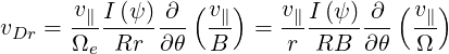
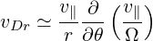
Using expressions (3.31), (3.32) and (3.58) or (3.72), we obtain in steady-state
 | (3.82) |
which can be rewritten as
 | (3.83) |
with
 | (3.84) |
![-1-∂- ^
B = R ∂s (RA ϕ)ψ
|∇ ψ |∂
- --------(RA ϕ)^s
[R ∂ψ ( )]
+ |∇ψ |-∂-(As) - |∇ ψ | ∂- -A-ψ- ^ϕ (3.44)
∂ψ ∂s |∇ ψ|](NoticeDKE258x.png)