= 1 which correspond to
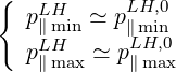
the condition
= 1 which correspond to
the condition
Internal boundaries
Momentum dynamics is described in spherical coordinates, because collisions is the dominant
physical process for current drive and matrices are therefore expected to be well conditionned.
Consequently, internal boundaries must be specified at p = 0 and = 1 which correspond to
the condition
 | (5.459) |
Here Neumann type boundary conditions are used, and therefore only gradients must be specified at the
internal boundaries4.
One must thus determine  at p = 0 and
  = 1 for the flux grid only, since the
distribution and flux grids are interlaced by definition. Therefore, starting from grids definition
given in Sec. 5.2,
= 1 for the flux grid only, since the
distribution and flux grids are interlaced by definition. Therefore, starting from grids definition
given in Sec. 5.2,
 | (5.460) |
as Δξ0,1∕2 = Δξ0,-1∕2, ξ0,1∕2 =  et ξ0,0 = -1.
Much in the same way,
 | (5.461) |
since Δξ0,nξ+1∕2 = Δξ0,nξ-1∕2. Furthermore, since by definition,
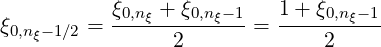 | (5.462) |
one obtains finally
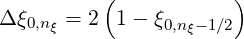 | (5.463) |
A similar technique may be used for the momentum grid p. Hence
 | (5.464) |
using Δp-1∕2 = Δp1∕2. Since Δp1∕2 = p1 - p0, and p1∕2 =  one obtains finally,
 | (5.465) |
because p0 = 0.
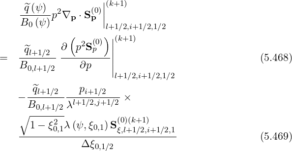
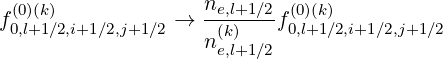
It is important to note that internal boundary conditions are only needed in the evaluation of the cross-derivative terms, since in the discrete form of the Fokker-Planck equation using two grids, as shown, in Sec. 5.4.1, they are automatically fullfiled for other terms. Indeed, at fixed ψl+1∕2,
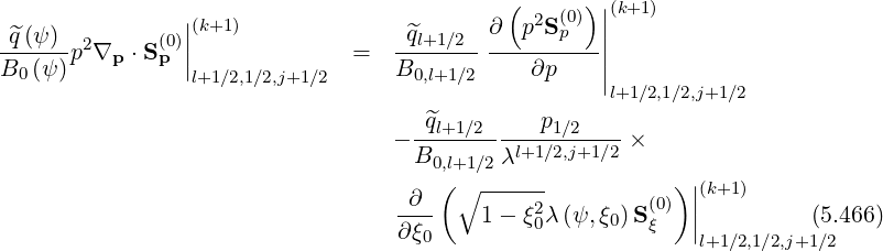
since p02Sp,l+1∕2,0,j+1∕2
 (k+1) = 0 with the flux grid here considered, at p0 = 0. In a similar way,
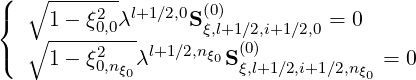 | (5.471) |
with ξ0,02 = ξ0,nξ 02 = 1
External boundaries
The other boundaries are inserted into the problem in violation of the true physical picture,
mainly because the momentum domain extends off to infinity, while only a subspace is
considered in computations. The upper limit of the domain is therefore chosen so that the
interesting physics may be accurately described, i.e. pmax ≫ pth for studying the Maxwellian
distribution function, pmax ≫ γ max for the RF waves and pmax ≫ pDreicer for the runaway
electrons. These conditions must ensure the conservative nature of the problem here addressed,
i.e. that plasma cannot enter or leave the domain of integration. This corresponds to the local
condition
max for the RF waves and pmax ≫ pDreicer for the runaway
electrons. These conditions must ensure the conservative nature of the problem here addressed,
i.e. that plasma cannot enter or leave the domain of integration. This corresponds to the local
condition
 | (5.472) |
where  is the normal to the external boundary. Because of the symmetry of the collision
operator, the subspace considered for computations is a sphere of radius pmax,
is the normal to the external boundary. Because of the symmetry of the collision
operator, the subspace considered for computations is a sphere of radius pmax,  =
=  . When the
condition (5.472) is fullfiled, external boundary conditions have almost a negligible influence,
and the numerical solution in the subspace is usually close to the theoretical one. It is usually
the case for most RF problems except for the Lower Hybrid wave in very hot plasmas, since the
range of resonant interaction between the wave and the electrons is well localized in momentum
space, far enough from the boundary so that no electron can leave the domain of
integration.
. When the
condition (5.472) is fullfiled, external boundary conditions have almost a negligible influence,
and the numerical solution in the subspace is usually close to the theoretical one. It is usually
the case for most RF problems except for the Lower Hybrid wave in very hot plasmas, since the
range of resonant interaction between the wave and the electrons is well localized in momentum
space, far enough from the boundary so that no electron can leave the domain of
integration.
The Fokker-Planck equation reduces to an hyperbolic equation in the vicinity of pmax (high
velocity limit), and therefore no boundary condition must be specified. In this condition, the
standard upstream differencing applies. Since for collisions, DppC ∕v ~ 1∕v4 and
FpC
∕v ~ 1∕v4 and
FpC ~ 1∕v2, one can consider that DppC
 ≈ 0 at p = pmax. Here, the pitch-angle scattering
term DξξC
≈ 0 at p = pmax. Here, the pitch-angle scattering
term DξξC requires no special handling, because it causes diffusion in a direction which is
parallel to the boundary.
requires no special handling, because it causes diffusion in a direction which is
parallel to the boundary.
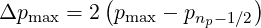
Nevertheless, since cross-derivative terms potentially involves points outside the computational domain, the following rule is used, even if the exact value of Δpmax has no specific importance,
 | (5.473) |
As by definition pnp+1∕2 =  =
=  , it results
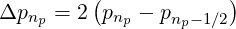 | (5.474) |
or in equivalent manner,
 | (5.475) |
Runaway electron problem
If an electric field is present, then in the real problem, some electrons will runaway and leave
the domain of integration. In that case, the condition Sp ⋅ = 0 is no more fullfiled, leading to
an effective loss of electrons. Since the Fokker-planck differential equation is of hyperbolic type,
no specific modification must be applied to the limit of the integration domain. However, one
must ensure that the total number of electrons is kept constant. Several techniques may be used
to avoid a decay of the number of electrons at the runaway rate ΓR
= 0 is no more fullfiled, leading to
an effective loss of electrons. Since the Fokker-planck differential equation is of hyperbolic type,
no specific modification must be applied to the limit of the integration domain. However, one
must ensure that the total number of electrons is kept constant. Several techniques may be used
to avoid a decay of the number of electrons at the runaway rate ΓR , as defined in Sec.
3.6.
, as defined in Sec.
3.6.
A possibility is to perform the following substitution
![[ ∫ t (0) ′ ]
f(00)(t,ψ,p,ξ0) → f0(0)(ψ,p,ξ0)exp - Γ-R-(ψ,t-)dt′
0 ne(ψ )](NoticeDKE3577x.png) | (5.476) |
in the Fokker-Planck equation, so that f0
 is independent of t. In that case, the
momentum matrix coefficients Mp,l+1∕2,i+1∕2,j+1∕2
is independent of t. In that case, the
momentum matrix coefficients Mp,l+1∕2,i+1∕2,j+1∕2 must be modified according to the
prescription
must be modified according to the
prescription
 | (5.477) |
where ΓR,l+1∕2
 is the runaway rate calculated at ψl+1∕2 and time step k as defined in Sec.
5.2. As a consequence, the Fokker-Planck equation becomes slightly non-linear, since
ΓR,l+1∕2
is the runaway rate calculated at ψl+1∕2 and time step k as defined in Sec.
5.2. As a consequence, the Fokker-Planck equation becomes slightly non-linear, since
ΓR,l+1∕2
 is an integral over the distribution function f0
 determined at time step k.
However, since the runaway population is usually very small as compared to the bulk, the
non-linearity remains fairly weak. Nevertheless, this approach has two major drawbacks: the
Fokker-Planck equation has no more an intrinsic conservative form, and in addition
matrix Mp
determined at time step k.
However, since the runaway population is usually very small as compared to the bulk, the
non-linearity remains fairly weak. Nevertheless, this approach has two major drawbacks: the
Fokker-Planck equation has no more an intrinsic conservative form, and in addition
matrix Mp must be recalculated at each time step, since it is time dependent. All
the advantages of the numerical implicit time scheme for a fast and stable rate of
convergence are therefore lost. For this reason, this method is not considered in the
code.
must be recalculated at each time step, since it is time dependent. All
the advantages of the numerical implicit time scheme for a fast and stable rate of
convergence are therefore lost. For this reason, this method is not considered in the
code.
Another technique is to inject cold electrons at p = 0, in order to compensate runaway losses
and keep the electron density constant at ψl+1∕2. Such an approach has the main advantage to
have a clear physical meaning. Indeed, the loss of electrons will generate locally an electric field
which in turn will force a flux of particles to compensate this local depletion. By definition,
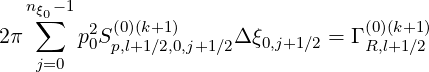
the number of electrons leaving the integration domain is simply ΓR . In principle,
without particle losses, p02Sp,l+1∕2,0,j+1∕2
. In principle,
without particle losses, p02Sp,l+1∕2,0,j+1∕2 = 0, though Sp,l+1∕2,0,j+1∕2
 is infinite at
p = 0, since, by definition, the Maxwellian distribution is an exact eigenfunction of the
Fokker-Planck operator. Compensation of hot electron losses by cold ones leads to the
relation
is infinite at
p = 0, since, by definition, the Maxwellian distribution is an exact eigenfunction of the
Fokker-Planck operator. Compensation of hot electron losses by cold ones leads to the
relation
 | (5.478) |
By definition, Sp,l+1∕2,0,j+1∕2
 is assumed uniform in pitch-angle, since no specific
direction can be physicaly priviledged. Therefore,
is assumed uniform in pitch-angle, since no specific
direction can be physicaly priviledged. Therefore,
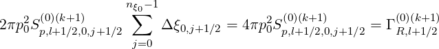 | (5.479) |
and
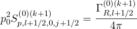 | (5.480) |
for all j values.
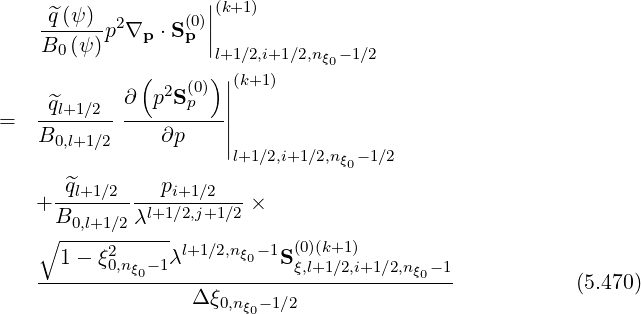
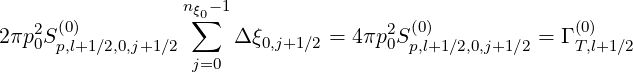
Expression (5.467) is then modified according to the relation
Since ΓR,l+1∕2 (k+1) is a weak function of f0
 , it is possible to replace ΓR,l+1∕2
 (k+1) by
its explicit form ΓR,l+1∕2
(k+1) by
its explicit form ΓR,l+1∕2 (k), so that one may avoid to recalculate matrix Mp,l+1∕2,i+1∕2,j+1∕2
 at each iteration, an extremely time consuming procedure. Consequently, with this scheme, the
zero order Fokker-Planck equation becomes simply
at each iteration, an extremely time consuming procedure. Consequently, with this scheme, the
zero order Fokker-Planck equation becomes simply
The condition to maintain density constant at each radial location ψl+1∕2 leads therefore to an additional term, that adds to the operator which describes damping of Maxwellian electrons on suprathermal ones. With this approach, the Fokker-Planck equation is slightly non-linear, provided the fraction of runaway electrons remain small as compared to the bulk one.
Furthermore, the electron distribution function is not a Maxwellian in the vicinity of p = 0,
since an ad-hoc source term of particle with no velocity is added. This approach is therefore
questionable for its validity, owing to the basic assumptions that are used to derive the
linearized Fokker-Planck equation around a Maxwellian bulk. Therefore, in order to avoid this
singularity, an alternative approach may be to add a source term normalized to ΓR,l+1∕2 (k)
but, whose distribution function is an exact Maxwellian corresponding to the electron
temperature at ψl+1∕2.
(k)
but, whose distribution function is an exact Maxwellian corresponding to the electron
temperature at ψl+1∕2.
In that case, in steady-state regime, the flux divergence ∇p ⋅ Sp is no more null at each
plasma location, but is given by the relation
is no more null at each
plasma location, but is given by the relation
![| Γ (0)(k) [ p2 ]
p2∇p ⋅S (0p)||(k+1) = p2 [---R,l+1∕2]---exp - (---------i+1∕2-)-------
l+1∕2,i+1∕2,j+1∕2 i+1∕2 2πTe,l+1∕23∕2 1 + γl+1∕2,i+1∕2 Te,l+1∕2](NoticeDKE3607x.png) | (5.484) |
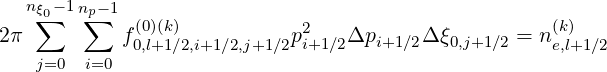
where Te = Te,l+1∕2, which corresponds to the existence of an external Maxwellian
source term. By definition,
= Te,l+1∕2, which corresponds to the existence of an external Maxwellian
source term. By definition,
2π ∑
j=0nξ0-1 ∑
i=0np-1![Γ (0)(k)
[----R,l+1∕2]---
2πTe,l+1∕2 3∕2](NoticeDKE3609x.png) exp exp![[ p2 ]
- (---------i+1∕2-)-------
1 + γl+1∕2,i+1∕2 Te,l+1∕2](NoticeDKE3610x.png) | |||
× pi+1∕22Δp
i+1∕2Δξ0,j+1∕2 = ΓR,l+1∕2 (k) (k) | (5.485) |
and the Fokker-Planck equation becomes simply
![f(0)(k+1) - f(0)(k)
-^ql+1∕2-p2 -0,l+1∕2,i+1∕2,j+1∕2----0,l+1∕2,i+1∕2,j+1∕2
B0,l+1∕2 i+1∕2 Δt
||(k+1)
+ -^q-p2∇p ⋅ S(0p)||
B0 l+1∕2,i+1∕2,j+1∕2
||(k+1)
+ -^q-p2∇ ψ ⋅S(ψ0)||
B0 l+1∕2,i+1∕2,j+1∕2
2 (0)(k) [ 2 ]
- -^ql+1∕2--pi+1∕2ΓR,l+1∕2exp - (--------pi+1∕2-)-------
B0,l+1∕2[2πTe,l+1∕2]3∕2 1+ γl+1∕2,i+1∕2 Te,l+1∕2
= 0 (5.486)](NoticeDKE3612x.png)
Though this technique is in principle the most consistent with the underlying physics, it has also still some numerical drawbacks, because of the forward time differencing. It is well known that such terms put strong limitations on the time step value Δt, in order to preserve numerical stability. A coarse estimate of its level can be deduced from the condition
![Γ (0)(k) [ p2 ] f (0)(k)
[----R,l+1∕2]---exp - (---------i+1∕2)-------- ≪ -0,l+1∕2,i+1∕2,j+1∕2
2πTe,l+1∕2 3∕2 1+ γl+1∕2,i+1∕2 Te,l+1∕2 Δt](NoticeDKE3613x.png) | (5.487) |
Assuming f0,l+1∕2,i+1∕2,j+1∕2 (k) ≃ f0M,l+1∕2,i+1∕2,j+1∕2
 , it turns out that
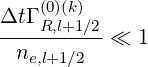 | (5.488) |
where ne,l+1∕2 = ne is the local electron density. In normalized units, as defined in
Sec.6.3, time step of the order of Δt ~ 10+3 - 10+4 are used to reach in few iterations the
steady-state solution. Therefore, ΓR,l+1∕2
is the local electron density. In normalized units, as defined in
Sec.6.3, time step of the order of Δt ~ 10+3 - 10+4 are used to reach in few iterations the
steady-state solution. Therefore, ΓR,l+1∕2 (k)∕ne,l+1∕2 must be lower than 10-5 - 10-6 in order
to avoid onset of numerical instabilities, which corresponds usually to normalized Ohmic electric
field less than 0.05.
(k)∕ne,l+1∕2 must be lower than 10-5 - 10-6 in order
to avoid onset of numerical instabilities, which corresponds usually to normalized Ohmic electric
field less than 0.05.
Finally, the ultimate and most simple approach to deal with the loss of runaway electrons is to enforce the electron distribution function at each time step. Defining a numerical density ne,l+1∕2(k) at time step k ,
 | (5.489) |
this procedure corresponds to the following replacement
 | (5.490) |
This procedure is equivalent to reinject electrons in the plasma so that local density is steadily maintained. The main advantage of this method is that it preserves the implicit or backward numerical time advancing. Furthermore, it avoids flux calculations in order to determine the runaway rate at ech time step, a procedure which slows down the rate of convergence. Finally, the normalization procedure is general and may be applied for any process that leads to local electron losses, like radial transport, magnetic ripple losses. For this reason, this method is chosen, if needed, for the code. However, even if this technique is numericaly very powerful, and physicaly justified, it may hinder some artificial numerical electron losses resulting from an improper numerical flux balance in each cell. Consequently, it is crucial to benchmark the Fokker-Planck code without this option, in order to verify that the conservative scheme is well satisfied and that electron losses remain always small.
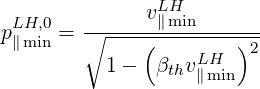
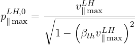
Lower hybrid wave and very high temperature plasmas For the Lower Hybrid current drive problem, difficulties similar to the runaway problem may take place in the core region of the plasma, when the electron temperature is very high. For this quasi-electrostatic wave, the resonant interaction with the plasma takes place along the magnetic field line, as discussed in Sec. 4.3.2, and therefore, a tail of very energetic electrons is pulled out from the bulk in the parallel direction p∥ as for the Ohmic electric field. Unlike the Ohmic case, the domain of interaction for the Lower Hybrid wave is bounded in momentum space, and is given by the well known wave-particle resonance condition
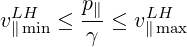 | (5.491) |
where the relativistic factor γ =  , β
th = vth∕c and p2 = p
∥2 + p⊥2. On the axis
p⊥ = 0, the resonance domain is given by the relation
, β
th = vth∕c and p2 = p
∥2 + p⊥2. On the axis
p⊥ = 0, the resonance domain is given by the relation
 | (5.492) |
where
 | (5.493) |
and
 | (5.494) |
When p⊥≠0, the lower bound of the resonance condition becomes
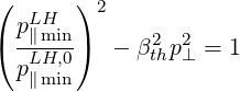 | (5.495) |
while the upper limit is
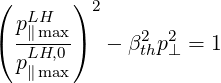 | (5.496) |
For very cold plasmas, i.e. when βth2pmax2 ≪ 1 since p⊥≤ pmax,
 | (5.497) |
and resonance domain boundaries are straight lines parallel to p∥ = 0 axis. In that case, electron losses are naturally very weak, since at the intersection of the resonance and integration domains, the wave-induced flux is nearly tangent to the boundary of the integration domain. Since pmax ranges usualy between 20 - 30, βth must be much less than 0.01, which corresponds to electron temperatures less than 0.06keV . Such a condition is never encountered in tokamak plasmas, except close to the very edge.
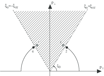
Because of relativistic corrections, lower and upper boundaries of the Lower Hybrid resonance domain are hyperbolic functions of p⊥, which indicates that the wave induced particle flux always crosses the integration domain. The curvature of the resonance domain boundaries as a function of p⊥ depends directly of βth as shown in Fig. 5.3 and therefore, one may expect that particle flux induced by the wave may be nearly perpendicular to the integration domain boundary. This is the worst situation, for which important losses of electrons may take place if the quasilinear diffusion is very large between p∥ minLH and p∥ maxLH, as for the runaway problem. In such a regime, a tail of very energetic electrons is pulled out from the bulk up to the integration domain, and the accuracy of the current driven by the wave as calculated by the code is highly questionable, when a significant fraction of this population leaves the integration domain.
This difficulty becomes rapidly important when βth increases as a consequence of the forward peaking of the electron dynamic because of the relativistic corrections. In that case, the total kinetic energy comes into play, and therefore electrons with a high p⊥ component will interact resonantly with the wave at larger p values because of their increasing mass.
It is difficult to introduce an unambiguous criterion which defines limits beyond which electron losses become important, since there is an interplay between the shape of the resonant domain, and also the absolute level of the quasilinear diffusion rate. As discussed in Sec. 4.3.2, its value is given by the relation
![-- θb 2 -- | |2
DRFb,n(0)(p,ξ0) = γpT-e-1-rθb-B---ξ0Ψ θbDRFb,,n,θ0b||Θb,n (kb)|| ×
p |ξ0|λ^q R0 BθPbξ2θb k,θb
[ ∑ ] ( )
H (θb - θmin)H (θmax - θb) 1- δ N ∥b - N θb (5.498)
2 σ T ∥res](NoticeDKE3629x.png)
As shown in Fig. 5.3, the only possibility for particle losses to remain at an acceptable small
level whatever the quasilinear diffusion level, is that the upper boundary of the Lower Hybrid
resonance domain crosses the integration domain at p⊥∕pmax > 1∕ . This purely geometrical
effect put very strong limitations on the lowest level of the parallel refractive index
n∥ minLH that can be studied. Indeed, , p∥ maxLH,0
. This purely geometrical
effect put very strong limitations on the lowest level of the parallel refractive index
n∥ minLH that can be studied. Indeed, , p∥ maxLH,0 is therefore given by the
relation,
is therefore given by the
relation,
 | (5.499) |
or
 | (5.500) |
In term of parallel refractive wave index, the previous condition is equivalent to the simple relation
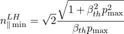 | (5.501) |
where the usual resonance relation
 | (5.502) |
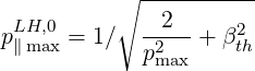
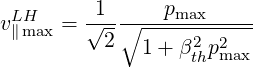
is used. In the limit βth2pmax2 ≫ 1, v∥ maxLH becomes independent of pmax
 | (5.503) |
which equivalent to
 | (5.504) |
This result confirms that increasing pmax is useless in order to reduce particle losses, if the quasilinear diffusion coefficient Db,nLH(0) remains very large over all the quasilinear resonance domain, except if the parallel refractive index is small. In most calculations, pmax ≃ 20 - 30, and since in the core of the plasma βth ranges between 0.14 and 0.17, βth2pmax2 ≃ 7.8 - 26, which fully justify this approximation.
As discussed for the runaway problem, particle losses are compensated by the normalization
of the electron distribution function at each time step. However, when n∥ minLH exceeds  , a
warning is send by the code, in order to indicate that strong particle losses may take
place if the quasilinear diffusion coefficient is large at the boundary of the integration
domain.
, a
warning is send by the code, in order to indicate that strong particle losses may take
place if the quasilinear diffusion coefficient is large at the boundary of the integration
domain.
Treatment of the trapped region
Since characteristic times for collision, RF quasilinear diffusion and Ohmic electric field
acceleration are all much larger than the bounce time in the weak collision “banana” regime,
f0
 = f0
= f0
 when
when  ≤ ξ0T . Therefore, symmetrically place points around
ξ0 = 0 are equivalent in the trapped region, a physical property that is described by the term
≤ ξ0T . Therefore, symmetrically place points around
ξ0 = 0 are equivalent in the trapped region, a physical property that is described by the term
![[ ∑ ]
12 σ](NoticeDKE3644x.png) T in the bounce averaging procedure in Sec. 2.2.1. This effect introduces a new internal
boundary corresponding to the trapped-passing transition, and an external one at ξ0 = 0, since
by symmetry,
T in the bounce averaging procedure in Sec. 2.2.1. This effect introduces a new internal
boundary corresponding to the trapped-passing transition, and an external one at ξ0 = 0, since
by symmetry,
 | (5.505) |
The Fokker-Planck equation is then solved in a reduced domain of integration,
where the momentum phase space corresponding to -ξ0T ≤ ξ0 ≤ 0 is removed. Once
determined in this reduced domain, the distribution function is recovered on the whole
space, by enforcing the condition f0
 = f0
= f0
 in the interval
 ≤ ξ0T .
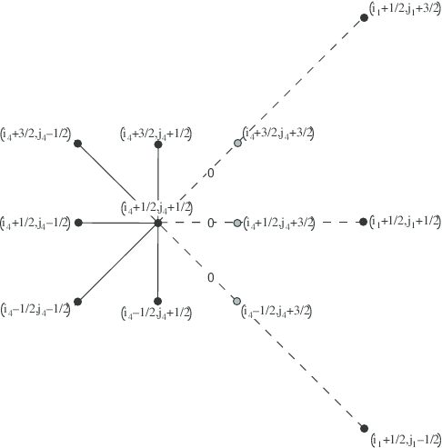
A specific treatment of the new internal boundary must be considered, so that flux continuity is correctly described between co- and counter-passing regions, despite the reduction of the phase space domain. Let define grid points
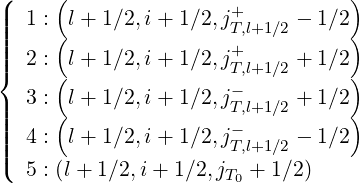 | (5.506) |
where jT0 =  ∕2 =
∕2 =  ∕2, as indicated in Fig.5.4. Here jT,l+1∕2-
is the index that corresponds to the trapped/passing boundary ξ0 = -ξ0T , while
jT,l+1∕2+ corresponds to the symmetric boundary with respect to the axis ξ0 = 0, i.e.
ξ0 = ξ0T .
∕2, as indicated in Fig.5.4. Here jT,l+1∕2-
is the index that corresponds to the trapped/passing boundary ξ0 = -ξ0T , while
jT,l+1∕2+ corresponds to the symmetric boundary with respect to the axis ξ0 = 0, i.e.
ξ0 = ξ0T .
By definition, grid points 1 and 3 are in the trapped region, just placed below and above co- and counter-passing boundaries respectively at opposite sides of the axis ξ0 = 0 and with the same distance to this axis, while grid points 2 and 4 have a similar arrangement but are placed in the co- and counter-passing regions respectively right after the trapped-passing boundary. The grid point 5 is placed on the right side of the axis ξ0 = 0, in the trapped sub-domain 0 ≤ ξ0 ≤ ξ0T .
Before performing the reduction of the domain of integration, the symmetry inside the trapped region must be enforced according to the relation
 | (5.507) |
where jT0 =  ∕2, with jT,l+1∕2- < j- < jT0 or an in equivalent manner jT0 < j+ <
jT,l+1∕2+. This procedure allows to correctly account for some processes that are not symmetric
in p∥, like wave-particle interaction.
∕2, with jT,l+1∕2- < j- < jT0 or an in equivalent manner jT0 < j+ <
jT,l+1∕2+. This procedure allows to correctly account for some processes that are not symmetric
in p∥, like wave-particle interaction.
The reduction of the domain of integration in the momentum phase space leads to introduce
a new matrix,  p
p whose coefficients are defined as follows
 | (5.508) |
with j′ = j, when 0 ≤ j < jT,l+1∕2-, and j′ = j - nξ0T,l+1∕2, when jT0 ≤ j ≤ nξ0 - 1. Here,
nξ0T,l+1∕2 =  ∕2 corresponds to the number of grid points removed in the
pitch-angle direction, and with this definition, it can be easily cross-checked that
jT0 - nξ0T,l+1∕2 = jT,l+1∕2-.
∕2 corresponds to the number of grid points removed in the
pitch-angle direction, and with this definition, it can be easily cross-checked that
jT0 - nξ0T,l+1∕2 = jT,l+1∕2-.
Furthermore, since grid point 3 is no more considered in the calculations while grid points 3
and 1 are equivalent, flux relations between neighboring grid points 4 and 3 must then be
replaced by new relations wich link grid points 4 and 1. Much in the same way, flux relations
between grid points 2 and 3 no more exist, and therefore, the flux relation between grid points 2
and 1 must be modified accordingly. This procedure leads to add six new set of coefficients to
the matrix  p
p , namely
![(
|| ^-(0) [ ]
|||{ M p,l+1∕2,i-1∕2, j′T-,l+1∕2- 1∕2 +nξ0T,l+1∕2
^-(0) [ ]
|| M p,l+1∕2,i+1∕2, j′T-,l+1∕2- 1∕2 +nξ0T,l+1∕2
|||( ^-(0) [ ]
M p,l+1∕2,i+3∕2, j′T-,l+1∕2- 1∕2 +nξ0T,l+1∕2](NoticeDKE3662x.png) | (5.509) |
and
![(
|| ^-(0) [′+ ]
|||{ M p,l+1∕2,i-1∕2, jT,l+1∕2- 1∕2 -nξ0T,l+1∕2
^-(0) [′+ ]
|| M p,l+1∕2,i+1∕2, jT,l+1∕2- 1∕2 -nξ0T,l+1∕2
|||( ^-(0) [ ]
M p,l+1∕2,i+3∕2, j′T+,l+1∕2- 1∕2 -nξ0T,l+1∕2](NoticeDKE3663x.png) | (5.510) |
while matrix coefficients
![(
| ^--(0) [ ]
|||| M p,l+1∕2,i-1∕2,j′-T,l+1∕2-1∕2+1
{ ^--(0) [ ]
| M p,l+1∕2,i+1∕2,j′-T,l+1∕2-1∕2+1
|||| ^--(0) [ ]
( M p,l+1∕2,i+3∕2,j′-T,l+1∕2-1∕2+1](NoticeDKE3664x.png) | (5.511) |
and
![(
|| ^--(0) [ ]
||| M p,l+1∕2,i-1∕2,j′+T,l+1∕2-1∕2+1
{ ^--(0) [ ]
|| M p,l+1∕2,i+1∕2,j′+T,l+1∕2-1∕2+1
||| ^--(0) [ ]
( M p,l+1∕2,i+3∕2,j′+T,l+1∕2-1∕2+1](NoticeDKE3665x.png) | (5.512) |
where jT,l+1∕2′- = jT,l+1∕2- and jT,l+1∕2′+ = jT,l+1∕2+ - nξ0T,l+1∕2 must be modified accordingly.
As shown in a graphic form in Figs. 5.5 and 5.6,
![(
|| ^--(0) [ ]
||| M p,l+1∕2,i-1∕2,j′-T,l+1∕2-1∕2+1 = 0
{ ^--(0) [ ]
|| M p,l+1∕2,i+1∕2,j′-T,l+1∕2-1∕2+1 = 0
||| ^--(0) [ ]
( M p,l+1∕2,i+3∕2,j′-T,l+1∕2-1∕2+1 = 0](NoticeDKE3666x.png) | (5.513) |
since the distribution function at grid 4 is no more connected with the one at grid point 3 or 5, but to the grid point 1 only. Furthermore, since grid points 1 and 3 are equivalent, their clockwise flux links with grid point 2 are only half in order to avoid counting them twice. Therefore,
![^--(0) [ ] --(0) [ ]
M p,l+1∕2,i-1∕2,j′+T,l+1∕2-1∕2+1 = M p,l+1∕2,i- 1∕2,j′T+,l+1∕2-1∕2 +1+nξ0T,l+1∕2∕2
---(0) ---
^M p,l+1∕2,i+1∕2,[j′+ -1∕2]+1 = M (0) [+ ] ∕2
T,l+1∕2 p,l+1∕2,i+1 ∕2,jT,l+1∕2-1∕2 +1+nξ0T,l+1∕2
^--(0) [ ] --(0) [ ]
M p,l+1∕2,i+3∕2,j′+T,l+1∕2-1∕2+1 = M p,l+1∕2,i+3 ∕2,j+T,l+1∕2-1∕2 +1+nξ0T,l+1∕2∕2
(5.514)](NoticeDKE3667x.png)
Moreover, since counterclockwise flux that links grid points 3 and 4 is equivalent by symmetry with clockwise flux that links grid points 1 and 2 , one obtains,
![^-(0) [ ] --(0) [ ]
M p,l+1∕2,i-1∕2, j′T-,l+1∕2- 1∕2 +nξ0T,l+1∕2 = M p,l+1∕2,i-1∕2,jT′+,l+1∕2-1∕2 +1+nξ0T,l+1∕2
--(0) --(0)
^M p,l+1∕2,i+1∕2,[j′- - 1∕2]+n = M [ ′+ ]
T,l+1∕2 ξ0T,l+1∕2 p,l+1∕2,i+1∕2,jT,l+1∕2-1∕2 +1+nξ0T,l+1∕2
^-(0) [ ] --(0) [ ]
M p,l+1∕2,i+3∕2, j′T-,l+1∕2- 1∕2 +nξ0T,l+1∕2 = M p,l+1∕2,i+3∕2,jT′+,l+1∕2-1∕2 +1+nξ0T,l+1∕2
(5.515)](NoticeDKE3668x.png)
![^-(0) [ ] --(0) [ ]
M p,l+1∕2,i-1∕2, j′T+,l+1∕2- 1∕2 -nξ0T,l+1∕2 = M p,l+1∕2,i-1∕2,j′T+,l+1∕2-1∕2 +1+nξ0T,l+1∕2∕2
--(0) --(0)
^M p,l+1∕2,i+1∕2,[j′+ - 1∕2]-n = M [′+ ] ∕2
T,l+1∕2 ξ0T,l+1∕2 p,l+1∕2,i+1∕2,jT,l+1∕2-1∕2 +1+nξ0T,l+1∕2
^-(0) [ ] --(0) [ ]
M p,l+1∕2,i+3∕2, j′T+,l+1∕2- 1∕2 -nξ0T,l+1∕2 = M p,l+1∕2,i+3∕2,j′T+,l+1∕2-1∕2 +1+nξ0T,l+1∕2∕2
(5.516)](NoticeDKE3669x.png)
Finally, for the external boundary at ξ0 = 0, all matrix coefficients at grid point jT0 + 1∕2 are forced to zero, except two,
![^-(0) [ ]
M p,l+1∕2,i-1∕2, j′T- +1 ∕2 +nξ = 1
,l+1∕2 0T,l+1∕2
^-(0) [ ]
M p,l+1∕2,i-1∕2, j′T-,l+1∕2+3 ∕2 +nξ0T,l+1∕2 = - 1 (5.517)](NoticeDKE3670x.png)
Magnetic ripple losses Super-trapped electrons with p∥∕p⊥≪ 1 are very sensitive to all the details of the magnetic configuration, and may be lossed in the local magnetic wells because of the finite number of toroidal magnetic field coils. This effect requires in principle a full 3 -D spatial calculation, that is beyond the present theoretical frame here described, as for the stellarator magnetic configuration. Nevertheless, some interesting results may be obtained, by considering that super-trapped electrons whose banana tips fall in the magnetic well drift vertically in an irreversible manner and leave therefore the plasma. This process takes place provided their kinetic energy is large enough so that the detrapping probability by collisions remain negligible.
Describing this effect is consequently equivalent to introduce new external boundaries in the trapped region, in order to describe in an ad-hoc manner this physical effect. This approach is justified because the drifting time across the plasma is short enough for the locally trapped electrons in the magnetic ripple to neglect their contributions to the overall momentum dynamics.
cmcmcm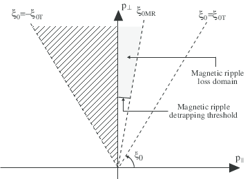
For this purpose, an Krook term is introduced in the Fokker-Planck equation
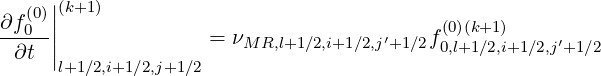 | (5.518) |
where νMR,l+1∕2,i+1∕2,j′+1∕2 is an effective loss frequency, whose value is a function of the super-trapped domain as shown in Fig. 5.7. This loss frequency varies therefore with the radial location ψl+1∕2, but also with momentum pi+1∕2 and pitch-angle ξ0,j′+1∕2. Outside this domain, νMR,l+1∕2,i+1∕2,j′+1∕2 is set to a zero so that losses are always negligible on the time scale for the steady-state distribution function to build-up. Conversely, inside the domain characterized by the pitch-angle boundary 0 ≤ ξ0,j′+1∕2 ≤ ξ0,jMR,l+1∕2′++1∕2 and pi+1∕2 ≥ pMR,l+1∕2, where jMR,l+1∕2′+ is the index below which particle are lossed in the magnetic ripple, and pMR,l+1∕2 is the momentum detrapping threshold by collisions, νMR,l+1∕2,i+1∕2,j′+1∕2 is usually taken constant and much larger than τt-1 which is the smallest time scale here considered, namely the transit time. The matrix is then simply modified according to the following rule
 | (5.519) |
With this method, it is not necessary to introduce additional specific conditions and moreover the implicit time scheme is fully preserved. By definition, the Fokker-Planck equation is no more conservative, but particle losses are compensated by the normalization technique at each time step, as for the runaway problem. This is an acceptable technique, provided level of losses due to magnetic ripple is small as compared to the electron bulk density.
Internal boundary For the dynamics in configuration space, since the problem has only one dimension, the internal boundary must be only specified at ψ = ψ0 = 0, which corresponds to the condition
 | (5.520) |
Using the same approach as for the momentum dynamics, Δψ must be defined at this location. Hence
 | (5.521) |
using Δψ-1∕2 = Δψ1∕2. Since Δψ1∕2 = ψ1 - ψ0, and ψ1∕2 =  one obtains finally,
 | (5.522) |
because ψ0 = 0.
It is important to note that internal boundary conditions are also only needed for the evaluation of cross-derivative terms, since in the discrete form of the Fokker-Planck equation using two grids, as shown, in Sec. 5.4.2, it is automatically fullfiled for other terms. Indeed, at fixed pi+1∕2,ξ0,j+1∕2,
 (k+1) = 0. Indeed, BP0,0 = 0 on the magnetic axis.
External boundary As discussed for the momentum dynamics, a primary condition of the code is that electron density profile is preserved. As for the particle losses in momentum space, this can be performed by injecting an equivalent number of particles at p = 0, in order to compensate the particle flux leaving the integration domain because of diffusion across magnetic flux surfaces. It corresponds to a reaction of the bulk, because of the occurence of a small electric field, generated by the electron transport so that the overall electron density profile is kept constant. By this method, a steady state regime may be achieved, and it is not necessary to specify which type of mechanism is at play, diffusion or convection.
Let define the local variation of the electron density Δne,l+1∕2 at time step k because of
spatial transport by the simple relation
at time step k because of
spatial transport by the simple relation
![∫∫ [ ]
Δn (ek)(ψ) = f(00)(k)(ψ, p,ξ0) - f(00)(k-1)(ψ,p,ξ0) λ(ψ, ξ0) p2dpdξ0](NoticeDKE3681x.png) | (5.525) |
It can be expressed in term of a loss rate
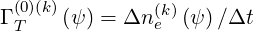
by introducing the integration time step Δt and the flux balance gives on the discrete mesh is
 | (5.526) |
assuming like for losses in momentum space that the flux has no pitch-angle dependence at p0. The zero order Fokker-Planck equation becomes simply
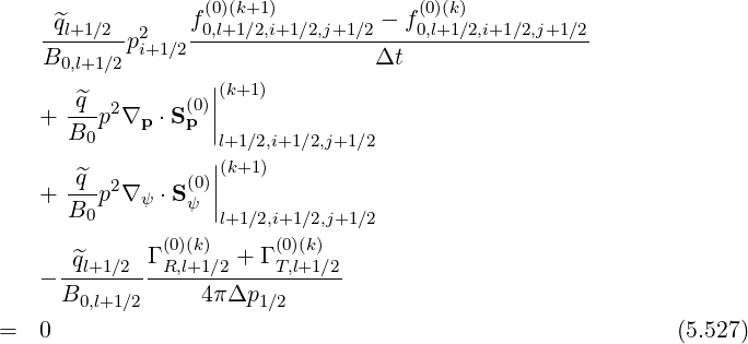
![f(0)(k+1) - f (0)(k)
-^ql+1∕2-p2i+1∕2-0,l+1∕2,i+1∕2,j+1∕2---0,l+1∕2,i+1∕2,j+1∕2
B0,l+1∕2 Δt
^q ||(k+1)
+ ---p2∇p ⋅S(p0)||
B0 l+1∕2,i+1∕2,j+1∕2
^q ||(k+1)
+ ---p2∇ψ ⋅S(ψ0)||
B0 l+1∕2,i+1 ∕2,j+1∕2
Γ (0)(k) + Γ (0)(k) [ p2 ]
--^ql+1∕2-p2 --R[,l+1∕2---T,]l+1-∕2 exp -(---------i+1∕2)-------
B0,l+1∕2 i+1∕2 2πTe,l+1∕2 3∕2 1 + γl+1∕2,i+1∕2 Te,l+1∕2
= 0 (5.528)](NoticeDKE3685x.png)
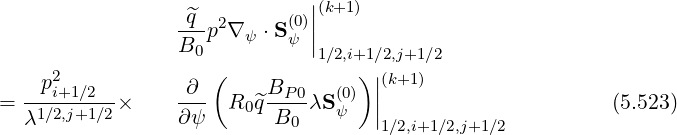
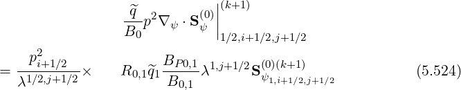
Finally, for cross-derivative terms, one have to determine Δψnψ at the boundary of the integration domain. It is readily given by relation,
 | (5.529) |
as done for p, since ψnψ = ψa.
Treatment of the trapped region The radial transport equation is greatly complicated by the presence of trapped electrons, since the diffusion across magnetic field lines may contribute to trap or detrap particles who are in the close vicinity of the trapped/passing boundary, because of the radial dependence of this boundary, as shown in Fig. 5.8. By definition, this process takes place intrinsically at fixed magnetic moment, a fundamental assumption of the flux conservative form of the bounce averaged Fokker-Planck equation, as shown in Sec.3.5.1.
The matrix build-up is therefore quite complex, since one has to take into account that counter-passing electrons may be trapped when they diffuse towards lower magnetic regions of the plasma, while conversely, trapped electrons may be detrapped by crossing magnetic flux surfaces in the high magnetic field side direction.
Let define three neighboring grid points at radial locations ψl-1∕2, ψl+1∕2 and ψl+3∕2 and corresponding trapped/passing boundaries ξ0T,jT,l-1∕2±, ξ0T,jT,l+1∕2±, and ξ0T,jT,l+3∕2±, since non-uniform pitch-angle grid mesh is designed so that each boundary is exactly placed on the flux grid. By definition, since
 | (5.530) |
the following relation holds
 | (5.531) |
Here jT0 is the index of the grid point corresponding to the axis ξ0 = 0 in the trapped region at ψl+1∕2. This defines naturaly eight different regions in momentum space at ψl+1∕2, where spatial fluxes must be considered. Since matrix is reduced in momentum space, because the region jl+1∕2- < jl-1∕2- < jT0,l+1∕2 is not considered in the calculations, one has therefore to consider effectively only six regions, namely corresponding to
 | (5.532) |
and
 | (5.533) |
or using relations jT,l+1∕2′- = jT,l+1∕2- and jT,l+1∕2′+ = jT,l+1∕2+ - nξ0T,l+1∕2
 | (5.534) |
As for the momentum dynamics, the reduction of the domain of integration in the
momentum phase space leads to introduce a new matrix,  ψ
ψ . Obviously, the main diagonal is
fully preserved, and therefore
. Obviously, the main diagonal is
fully preserved, and therefore
 | (5.535) |
provided j′ < jT,l+1∕2′-, while
![--(0) --(0)
^M ψ,l+1∕2,i+1∕2,j′+1 ∕2 = M ψ,l+1∕2,i+1∕2,[j′+1∕2]+nξ
0T,l+1∕2](NoticeDKE3695x.png) | (5.536) |
when for j′ > jT,l+1∕2′+. Only off-diagonal matrix coefficients have to be modified, because of the presence of trapped and circulating electrons. Indeed, these coefficients reflect the particle flux transfer between different location.
If j′ < jT,l+3∕2′-, matrix coefficients are given by
 | (5.537) |
and for jT,l+3∕2′- < j′ < jT,l+1∕2′-, the simple relation still holds for one matrix coefficient only
 | (5.538) |
since the trapped region is narrower at ψl-1∕2 as compared to ψl+1∕2. But since counter-circulating electrons become trapped by diffusion from ψl+1∕2 → ψl+3∕2 and electron dynamics in the domain jT,l+3∕2- < j < jT0 is removed and replaced by its counterpart in the positive pitch-angle region jT0 < j < jT,l+3∕2+, it turns out that
 | (5.539) |
and the flux link must be replaced by
![^M--(0) ′ ′ = M--(0) ′
ψ,l+3∕2,i+1∕2,[j+1∕2]+2(jT0-(j +1∕2))-nξ0T,l+3∕2 ψ,l+3∕2,i+1 ∕2,j+1∕2](NoticeDKE3699x.png) | (5.540) |
taking into account of the mirror indexing around the axis ξ0 = 0, and the fact that matrix blocks corresponding to different radii have different sizes.
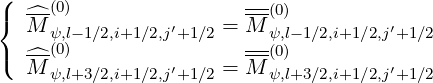
In a general way, when j′ > jT,l+1∕2′-, the following rule applies
 | (5.541) |
all corresponding matrix coefficients being replaced by new ones according to the relations
![( (0) ---
|{ ^M-- ′ ( ) = M-(0) ′
ψ,l-1∕2,i+1∕2,[j+1 ∕2]+ nξ0T,l+1∕2- nξ0T,l-1∕2 --ψ,l- 1∕2,i+1∕2,[j+1∕2]+nξ0T,l+1∕2
|( ^M-(0) ′ ( ) = M-(0) ′
ψ,l+3∕2,i+1∕2,[j+1 ∕2]+ nξ0T,l+1∕2- nξ0T,l+3∕2 ψ,l+3∕2,i+1∕2,[j+1∕2]+nξ0T,l+1∕2](NoticeDKE3701x.png) | (5.542) |
wether electrons remains trapped or co-passing, or become trapped by the outward radial transport or detrapped by the inward cross-field diffusion. Since nξ0T,l+1∕2 - nξ0T,l-1∕2 > 0 and nξ0T,l+1∕2 - nξ0T,l+3∕2 < 0,
![( ( )
{ ′ ′
[j + 1∕2]+ ( nξ0T,l+1∕2 - nξ0T,l-1∕2) > j + 1∕2
( [j′ + 1∕2]+ nξ0T,l+1∕2 - nξ0T,l+3∕2 < j′ + 1∕2](NoticeDKE3702x.png) | (5.543) |
which indicates that diagonals shrink when trapped/passing boundary is crossed, i.e.
j′ > jT,l+1∕2′-. Therefore, matrix  ψ
ψ contains much more diagonals than Mψ
 which has
only three ones.
which has
only three ones.
At ψ = 0, there is no need to specify the spatial flux Sψ , with the two grids technique.
Since by construction Rmin,0BP min,0Sψ0,i+1∕2,j+1∕2
, with the two grids technique.
Since by construction Rmin,0BP min,0Sψ0,i+1∕2,j+1∕2 (k+1) = 0, no particle accumulation occurs
naturaly at ψ , and at this singular point f0,1∕2,i+1∕2,j+1∕2
(k+1) = 0, no particle accumulation occurs
naturaly at ψ , and at this singular point f0,1∕2,i+1∕2,j+1∕2 (k+1) = f0,-1∕2,i+1∕2,j+1∕2
 (k+1) is
well fullfiled.
(k+1) is
well fullfiled.
At the plasma edge ψa, i.e. at the boundary of the integration domain, there is also no need to specify any condition on the flux of fast particles are leaving the plasma definitively, as for the runaway problem. Consequently, even without any external perturbation, the fact that radial transport of fast transport leads to strong departure from the Maxwellian momentum dependence at all radius.
As for the dynamics in momentum space, Δψ must be specified at the boundaries of the domain of integration. One finds that
 | (5.544) |
since ψ0 = 0, and
 | (5.545) |
noting that ψnψ = ψa.
Since the first order bounce-averaged drift kinetic equation may be expressed in the same
conservative form as for zero order Fokker-Planck bounce-averaged equation, most of the
boundary conditions apply in a natural way without additional specifications, in particular at
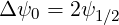
p = 0 and  = 1, as a consequence of the two grids technique, one for the fluxes and the other
for the distribution function.
= 1, as a consequence of the two grids technique, one for the fluxes and the other
for the distribution function.
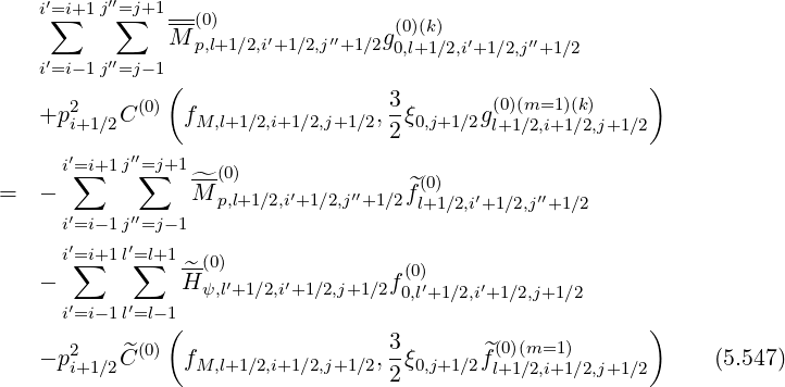
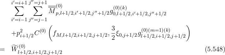
In matrix form, the general expression of the first order bounce averaged drift kinetic equation
 | (5.546) |
becomes
Here,  is the iteration index number, while C
 and
and 
 are the electron-electron
self-collision operators that make the equation non-linear.
are the electron-electron
self-collision operators that make the equation non-linear.

In the weak collision “banana” regime, it is shown in Sec.3.4 that g
 = 0 for trapped
electrons. Therefore, the drift kinetic equation must be solved in a reduced domain of
integration, as for f0
= 0 for trapped
electrons. Therefore, the drift kinetic equation must be solved in a reduced domain of
integration, as for f0
 , but with different and more simple internal boundary
conditions. Indeed, the only constraint is to enforce the condition g
, but with different and more simple internal boundary
conditions. Indeed, the only constraint is to enforce the condition g
 = 0 for
 ≤ ξ0T .
Let define grid points
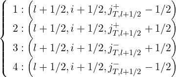 | (5.550) |
as indicated in Fig.5.9. Here jT,l+1∕2- is the index that corresponds to the trapped/passing boundary ξ0 = -ξ0T , while jT,l+1∕2+ corresponds to the symmetric boundary with respect to the axis ξ0 = 0, i.e. ξ0 = ξ0T .
Since g is prescribed in the trapped domain, all the region may be removed from
the calculations, and the reduction of the domain of integration in the momentum
phase space leads to introduce a new matrix
is prescribed in the trapped domain, all the region may be removed from
the calculations, and the reduction of the domain of integration in the momentum
phase space leads to introduce a new matrix  p
p whose coefficients are defined as
follows
whose coefficients are defined as
follows
 | (5.551) |
with j′ = j, when 0 ≤ j < jT,l+1∕2-, and j′ = j - mξ0T,l+1∕2, when jT,l+1∕2+ < j ≤ nξ0. Here, mξ0T,l+1∕2 = jT,l+1∕2+ - jT,l+1∕2- corresponds to the number of grid points removed in the pitch-angle direction, and with this definition, it is easy to cross-check that jT,l+1∕2′+ -jT,l+1∕2′- = jT,l+1∕2+ -jT,l+1∕2--mξ0T,l+1∕2 = 0. Since grid points 2 and 4 are not connected, the following condition applies
![(
|| ^^ (0) [ ]
|||{ M p,l+1∕2,i-1∕2,j′T,l+1∕2-1∕2+1 = 0
^^ (0) [ ]
|| M p,l+1∕2,i+1∕2,j′T,l+1∕2-1∕2+1 = 0
|||( ^ (0) [ ]
M^ p,l+1∕2,i+3∕2,j′T,l+1∕2-1∕2+1 = 0](NoticeDKE3734x.png) | (5.552) |
and conversely
![(
|| ^^ (0) [ ]
||| M p,l+1∕2,i-1∕2,j′T,l+1∕2+1∕2-1 = 0
{ ^ (0) [ ]
| M^ p,l+1∕2,i+1∕2,j′T,l+1∕2+1∕2-1 = 0
|||| ^ (0) [ ]
( M^ p,l+1∕2,i+3∕2,j′T,l+1∕2+1∕2-1 = 0](NoticeDKE3735x.png) | (5.553) |
where jT,l+1∕2′- = jT,l+1∕2′+ = jT,l+1∕2′. As internal boundaries match already existing
diagonals of the matrix Mp,l+1∕2,i+1∕2,j+1∕2 ,
,  p,l+1∕2,i+1∕2,j′+1∕2
 remains a simple
nine diagonal matrix, and is therefore less complex than the 15 diagonals matrix
remains a simple
nine diagonal matrix, and is therefore less complex than the 15 diagonals matrix
 p,l+1∕2,i+1∕2,j′+1∕2
 corresponding to the Fokker-Planck equation.

Since no inversion is required for calculating the vector  l+1∕2,i+1∕2,j+1∕2
 , it is consequently
evaluated at all grid points, including those corresponding to trapped electron domain.
Consequently, the reduction along the pitch-angle direction that results from the condition
g
, it is consequently
evaluated at all grid points, including those corresponding to trapped electron domain.
Consequently, the reduction along the pitch-angle direction that results from the condition
g
 = 0 is only performed after the calculation of
  l+1∕2,i+1∕2,j+1∕2 over the full ξ0
grid. Once done, the prescription on the index number j′ that holds for the matrix
conversion
l+1∕2,i+1∕2,j+1∕2 over the full ξ0
grid. Once done, the prescription on the index number j′ that holds for the matrix
conversion
 | (5.554) |
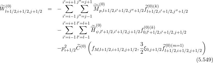
may be then applied in a similar way for  l+1∕2,i+1∕2,j+1∕2, which leads to define a new vector
 p,l+1∕2,i+1∕2,j′+1∕2
 whose size is reduced
 | (5.555) |
and finally the drift kinetic equation on the reduced grid is simply given by the relation
 | (5.556) |
where all the trapped electron domain is removed.
The problem of external boundaries discussed in Sec. 5.7.1 for the zero-order Fokker-Planck equation may be applied in a straightforward manner to the first-order drift kinetic ones, since it may be expressed in a similar conservative form. Consequently, if the zero-order Fokker-Planck equation conserves the total number of particles without specific conditions, the solution g may be found without additional constraints at the boundaries of the integration domain. Conversely, if Dirichlet conditions are considered for the Fokker-Planck equation, like enforcing the Maxwellian solution at p = 0, similar and consistent conditions must be also applied for the drift kinetic equation.