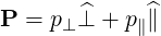
 along axes
  . The
vector position is momentum space is written
. The
vector position is momentum space is written
We consider a cartesian momentum space in coordinates along axes . The
vector position is momentum space is written
 | (A.208) |
We consider the two following curvilinear systems:

The coordinates  are defined on the space
| -∞≤ p∥ | < ∞ | (A.209) |
| 0 ≤ p⊥ | < ∞ | (A.210) |
| 0 ≤ φ | < 2π | (A.211) |
and is related to  by
by
| p∥ | = pz | (A.212) | |
| p⊥ | =  | ||
| φ | = arctan + πH + πH ![[2π]](NoticeDKE4833x.png) |
which is inverted to
| px | = p⊥cosφ | (A.213) | |
| py | = p⊥sinφ | ||
| pz | = p∥ |
The position vector in momentum space then becomes
 | (A.214) |
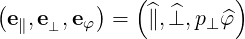
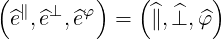
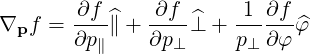
where we define a local orthonormal basis  as
as
 | =  | (A.215) |
 | = cosφ + sinφ + sinφ | (A.216) |
 | =  ∥× ∥× ⊥ = -sinφ ⊥ = -sinφ + cosφ + cosφ | (A.217) |
The covariant vector basis is defined in (A.1), which becomes here
| e∥ | =  = =  | (A.218) |
| e⊥ | =  = =  | (A.219) |
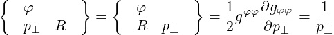
| eφ | =  = p⊥ = p⊥ = p⊥ = p⊥ | (A.220) |
so that we have the covariant basis
 | (A.221) |
the scaling factors
 | (A.222) |
and the normalized tangent basis
 | (A.223) |
The Contravariant vector basis is defined in (A.9), which becomes here
| e∥ | = ∇p
∥ =  | (A.224) |
| e⊥ | = ∇p
⊥ =  | (A.225) |
| eφ | = ∇φ =  | (A.226) |
The relations (A.10-A.11) are here readily verified. The normalized reciprocal basis is
 | (A.227) |
which here coincides with the normalized tangent basis, since both bases are orthogonal.
They are defined in (A.12) and become here
| gij | = 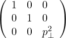 | (A.228) | |
| gij | = 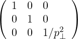 |
As a result
 | (A.229) |
and the Jacobian is
 | (A.230) |
dl | = dp∥ | (A.231) |
dl | = dp⊥ | (A.232) |
dl | = p⊥dφ | (A.233) |
dS | = p⊥dp⊥dφ | (A.234) |
dS | = p⊥dp∥dφ | (A.235) |
dS | = dp∥dp⊥ | (A.236) |
 | (A.237) |
They are defined in (A.49) and are all zero here except
 |
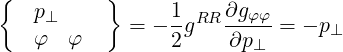 | (A.238) |
 | (A.239) |
 | (A.240) |
 ⋅ ⋅ | =    - -   | (A.241) |
 ⋅ ⋅ | =    - -  | (A.242) |
 ⋅ ⋅ | =   - -  | (A.243) |

The coordinates  are defined on the space
| 0 ≤ p | < ∞ | (A.244) |
| - 1 ≤ ξ | < 1 | (A.245) |
| 0 ≤ φ | < 2π | (A.246) |
and is related to  by
by
| p | = 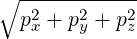 | (A.247) | |
| ξ | = 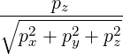 | (A.248) | |
| φ | = arctan + πH + πH ![[2π]](NoticeDKE4906x.png) |
which is inverted to
| px | = p cosφ cosφ | (A.249) | |
| py | = p sinφ sinφ | ||
| pz | = pξ |
Note that we have the following transformation from  to
to 
| p | =  | (A.250) | |
| ξ | =  |
which is inverted to
| p∥ | = pξ | (A.251) | |
| p⊥ | = p |
The position vector in momentum space then becomes
 | (A.252) |
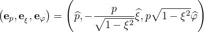
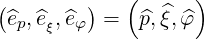
where we define a local orthonormal basis  as
as
 | =   + ξ + ξ | (A.253) |
 | =  × × = ξ = ξ - -  | (A.254) |
 | = -sinφ + cosφ + cosφ | (A.255) |
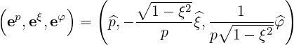
The covariant vector basis is defined in (A.1), which becomes here
| ep | =  = =  | (A.256) |
| eξ | =  = p = p = - = -  | (A.257) |
| eφ | =  = p = p = p = p  | (A.258) |
so that we have the covariant basis
 | (A.259) |
the scaling factors
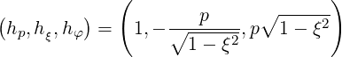 | (A.260) |
and the normalized tangent basis
 | (A.261) |
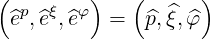
The Contravariant vector basis is defined in (A.9), which becomes here
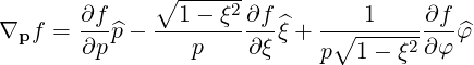
| ep | = ∇p =  = =  | (A.262) |
| eξ | = ∇ξ =  = - = -  | (A.263) |
| eφ | = ∇φ =  = =   | (A.264) |
The relations (A.10-A.11) are here readily verified. The reciprocal basis is
 | (A.265) |
and the normalized reciprocal basis is
 | (A.266) |
which here coincides with the normalized tangent basis, since both bases are orthogonal.
They are defined in (A.12) and become here
| gij | = 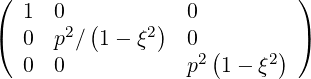 | (A.267) | |
| gij | = ![( )
1 0( 2) 2 0
( 0 1- ξ ∕p 0 [ ( )] )
0 0 1∕ p2 1- ξ2](NoticeDKE4953x.png) |
As a result
 | (A.268) |
and the Jacobian is
 | (A.269) |
dl | = dp | (A.270) |
dl | =  dξ dξ | (A.271) |
dl | = p dφ dφ | (A.272) |
dS | = p2dξdφ | (A.273) |
dS | = -p dpdφ dpdφ | (A.274) |
dS | =  dpdξ dpdξ | (A.275) |
 | (A.276) |
They are defined in (A.49) and are all zero here except
 | (A.277) |
 | (A.278) |
 ⋅ ⋅ | =    + +    | (A.279) | |
 ⋅ ⋅ | =    - -   | ||
 ⋅ ⋅ | = -   - -  |