
 limV →∞
 ∑
n=-∞∞
∑
n=-∞∞ d3k
d3k![[( [ 1 (k∥v∥ ) ] )
P*∥E *k,∥Jn + P *⊥ - --- ---* - 1 E *k,⊥
p⊥ ω](NoticeDKE2059x.png)
![]
--------i------ ( )
⋅[n Ω + k v - ω] Ek,∥JnP∥ + Ek,⊥P⊥ f
∥ ∥](NoticeDKE2060x.png)
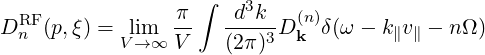
The volume-averaged quasilinear diffusion operator for radiofrequency waves in an infinite uniform plasma was first developped by Kennel and Engelmann [?]. The relativistic treatment was performed by Lerche [?], who proposes the following operator
| Q | = - limV →∞∑
n=-∞∞d3k | (4.188) | |
| |||
| |
with
| P∥ | =  - -  | (4.189) |
| P⊥ | =  + +   | (4.190) |
| Ek,⊥ | =   | (4.191) |
The electric field is assumed to be monochromatic at the frequency ω, and is decomposed into its Fourier components
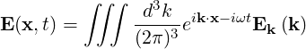 | (4.192) |
which are projected on the rotating field frame
| Ek,± | =   | (4.193) |
| Ek,∥ | = Ek,z | (4.194) |
The wave vector is expressed in cylindrical coordinates as
| kx | = k⊥cosα | (4.195) | |
| ky | = k⊥sinα | ||
| kz | = k∥ |
and the argument of the Bessel functions is k⊥v⊥∕Ω. The relativistic cyclotron frequency is
 | (4.196) |
In order to incorporate the RF wave physics in the Fokker-Planck or Drift Kinetic solvers, the operator (4.188) must be cast in a conservative form.
The transformation from cylindrical to spherical momentum derivatives is given by
 | =   + +   | (4.197) |
 | =   + +   | (4.198) |
Since
| p | =  | (4.199) |
| ξ | =  | (4.200) |
one obtains
 | = ξ | (4.201) |
 | =  | (4.202) |
 | =  | (4.203) |
 | = - | (4.204) |
Hence rewritting (4.189-4.190) in cylindrical coordinates using (4.197-4.198)
| P∥ | = ξ + +    | (4.205) |
| P⊥ | =   - -   | (4.206) |
In order to permute derivatives and the integral in expression (4.188) and obtain a
conservative formulation, one must express both P∥ and P⊥ in terms of the derivatives
associated with the divergence of a flux: 1∕p2 p2 and -1∕p
 .
.
Since
ξ | =   p2ξ - p2ξ - | (4.207) |
  | =   p2 p2 - - | (4.208) |
and
   | = -   + +  | (4.209) | |
-   | = -    | ||
+   + +  | (4.210) |
the operators in (4.188) can be expressed in a divergence form
| P∥ | =   p2ξ - p2ξ -   | (4.211) |
P⊥-  | =   p2 p2 - -    | (4.212) |
so that (4.188) can be rewritten as
 | (4.213) |
with
| SpRF | = limV →∞  ∑
n=-∞∞ ∑
n=-∞∞ d3k d3k | ||
![]
i ( )
⋅[n-Ω-+-k-v---ω-] Ek,∥JnP∥ + Ek,⊥P ⊥ f
∥ ∥](NoticeDKE2149x.png) | (4.214) |
| SξRF | = limV →∞  ∑
n=-∞∞ ∑
n=-∞∞ d3k d3k | ||
 | |||
![]
⋅[------i------] (E J P + E P )f
nΩ + k∥v∥ - ω k,∥ n ∥ k,⊥ ⊥](NoticeDKE2154x.png) | (4.215) |
Considering the above expressions of the fluxes and the operators (4.205-4.206), RF-induced fluxes are purely diffusive, and therefore they are expressed as
 | (4.216) |
with
 | (4.217) |
Hence, using the expression of the gradient in spherical coordinates,
| SpRF | = -DppRF + DpξRF + DpξRF  | (4.218) |
| SξRF | = -DξpRF + DξξRF + DξξRF  | (4.219) |
with
| DppRF | = -limV →∞  ∑
n=-∞∞ ∑
n=-∞∞ d3k d3k | ||
![( ∘ ------ )]
⋅[------i------] ξE Jn + 1 - ξ2Ek,⊥
nΩ + k∥v∥ - ω k,∥](NoticeDKE2167x.png) | (4.220) | ||
| DpξRF | = limV →∞  ∑
n=-∞∞ ∑
n=-∞∞ d3k d3k | ||
![i ( 1 ( nΩ ) 1( k v ) ) ]
⋅[-------------] ∘------- 1- ξ2 - --- Ek,∥Jn - -- ξ2 - -∥-∥ Ek,⊥
nΩ + k∥v∥ - ω 1 - ξ2 ω ξ ω](NoticeDKE2172x.png) | (4.221) | ||
| DξpRF | = -limV →∞  ∑
n=-∞∞ ∑
n=-∞∞ d3k d3k | ||
 | |||
![( ∘ -----)]
⋅[------i------] Ek,∥Jn ξ + Ek,⊥ 1- ξ2
nΩ + k∥v∥ - ω](NoticeDKE2177x.png) | (4.222) | ||
| DξξRF | = limV →∞  ∑
n=-∞∞ ∑
n=-∞∞ d3k d3k | ||
 | |||
![i ( 1 ( nΩ ) 1( k v ) ) ]
⋅[-------------] ∘------- 1- ξ2 - --- Ek,∥Jn - -- ξ2 - -∥-∥ Ek,⊥
nΩ + k∥v∥ - ω 1 - ξ2 ω ξ ω](NoticeDKE2182x.png) | (4.223) |
In the limit of a resonant diffusion,
![1 ( )
[nΩ-+-k-v----ω] → iπ δ ω - k∥v∥ - nΩ
∥ ∥](NoticeDKE2183x.png) | (4.224) |
and using the resonance condition
 | (4.225) |
RF diffusion coefficients may be expressed in a simple form
| DppRF | = ∑
n=-∞∞ D
nRF D
nRF | (4.226) |
| DpξRF | = ∑
n=-∞∞-  DnRF DnRF | (4.227) |
| DξpRF | = ∑
n=-∞∞-  DnRF DnRF | (4.228) |
| DξξRF | = ∑
n=-∞∞  2D
nRF 2D
nRF | (4.229) |
where we define a diffusion coefficient
 | (4.230) |
Using (4.191), we can define
| Dk(n) | = e2 | ||
 2 2 | (4.231) |
so that (4.230) becomes
 | (4.232) |
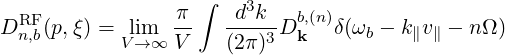
If rays are gathered in RF beams of different frequencies ωb, diffusion coefficients are sums of each contribution ower all hamonics n , leading to the expression
| DppRF | = ∑ n=-∞+∞∑ b(1 - ξ2)D b,nRF(p,ξ) | (4.233) |
| DpξRF | = ∑
n=-∞+∞∑
b - ![[ ]
1- ξ2 - nΩ-
ωb](NoticeDKE2201x.png) Db,nRF(p,ξ) Db,nRF(p,ξ) | (4.234) |
| DξpRF | = ∑
n=-∞+∞∑
b - ![[ nΩ ]
1- ξ2 - ---
ωb](NoticeDKE2203x.png) Db,nRF(p,ξ) Db,nRF(p,ξ) | (4.235) |
| DξξRF | = ∑
n=-∞+∞∑
b ![[ ]
2 nΩ-
1 - ξ - ωb](NoticeDKE2205x.png) 2D
b,nRF(p,ξ) 2D
b,nRF(p,ξ) | (4.236) |
where
 | (4.237) |
and Dkb,(n) accounts for the polarization and the intensity of the RF wave. It is given by
| Dkb,(n) | = e2 | ||
 2 2 | (4.238) |
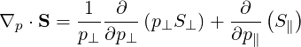
The Fokker-Planck equation is usually solved numerically in spherical coordinates, because of the spherical symmetry of the collisional operator. Therefore, in this coordinate system, the numerical problem is well-conditionned, ensuring stable convergence towards the solution. However, in many case the RF quasilinear operator has a more cylindrical symmetry, and it could be useful to derive its expression in this coordinate system, in order to get a more physical insight of the wave-particle interaction. Starting from the general expression of the flux divergence in cylindrical coordinates,
 | (4.239) |
and taking into account of the diffusive nature of the wave-particle interaction,
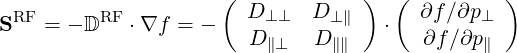 | (4.240) |
where the cylindrical tensor elements are related to the spherical ones by
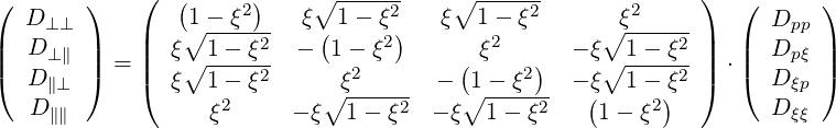 | (4.241) |
Applying this transformation, one obtains,
| D⊥⊥RF | = ∑
n=-∞+∞∑
b![[ ]
nΩ
ω--
b](NoticeDKE2212x.png) 2D
b,nRF(p,ξ) 2D
b,nRF(p,ξ) | (4.242) |
| D⊥∥RF | = ∑
n=-∞+∞∑
b  ![[ ]
1- nΩ-
ωb](NoticeDKE2215x.png) Db,nRF(p,ξ) Db,nRF(p,ξ) | (4.243) |
| D∥⊥RF | = ∑
n=-∞+∞∑
b  ![[ ]
1- nΩ-
ωb](NoticeDKE2218x.png) Db,nRF(p,ξ) Db,nRF(p,ξ) | (4.244) |
| D∥∥RF | = ∑
n=-∞+∞∑
b ![[ ]
nΩ-
1 - ω
b](NoticeDKE2220x.png) 2D
b,nRF(p,ξ) 2D
b,nRF(p,ξ) | (4.245) |
For n = 0 (which corresponds to the Lower Hybrid wave) the quasilinear diffusion is strictly along the parallel direction (i.e. magnetic field line). Also, at a cyclotron harmonic, where ωb = nΩ, the diffusion is only perpendicular, when relativistic corrections are not considered.
The quasilinear diffusion coefficient (4.230), describing the interaction of the electrons with a given beam b at an harmonic n, is rewritten as
 | (4.246) |
where,
Θkb, | =  ebk,+e-iαJ
n-1 ebk,+e-iαJ
n-1 + +  ebk,-e+iαJ
n+1 ebk,-e+iαJ
n+1 | ||
+  ebk,∥Jn ebk,∥Jn | (4.247) |
Here, the polarization vector in Fourier space
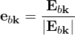 | (4.248) |
is introduced, whose components in the rotating field frame are
| ebk,+ | =  = = 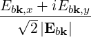 | (4.249) | |
| ebk,- | =  = =  | ||
| ebk,∥ | =  = =  |
The electric field associated with a given ray is described by a plane wave, with given frequency ωb and wave number kb:
Eb | = Re![[ ]
Eb0ei(kb⋅x-ωbt)](NoticeDKE2237x.png) = Re = Re![[ ]
^Eb](NoticeDKE2238x.png) | (4.250) |
=  ![[ ]
Eb0ei(kb⋅x-ωbt) + E*b0e-i(kb⋅x- ωbt)](NoticeDKE2240x.png) | (4.251) |
so that
Ebk | ≡ d3xe-ik⋅xE
b d3xe-ik⋅xE
b | ||
=  ![[ ∫ ∫∫ ∫∫ ∫ ]
Eb0e -iωbt d3xei(kb- k)⋅x + E *b0eiωbt d3xei(kb+k)⋅x](NoticeDKE2245x.png) | |||
=  ![[ - iωbt * iωbt ]
Eb0e δ(kb - k )+ E b0e δ(kb + k)](NoticeDKE2247x.png) | (4.252) |
The electric field is the sum of two contributions with different frequencies
Ebk+ | =  Eb0δ Eb0δ with ω = ωb with ω = ωb | (4.253) |
Ebk- | =  Eb0*δ Eb0*δ with ω = -ωb with ω = -ωb | (4.254) |
Therefore the QL diffusion tensor (4.217) is the sum of these two contributions:
 | (4.255) |
associated with the diffusion coefficients
| Db,nRF+(p,ξ) | = lim
V →∞    2 2 2δ 2δ | (4.256) | |
| Db,nRF-(p,ξ) | = lim
V →∞    2 2 2δ 2δ |
with, using (4.247)
Θkb+, | =  eb+k,+e-iαJ
n-1 eb+k,+e-iαJ
n-1 + +  eb+k,-e+iαJ
n+1 eb+k,-e+iαJ
n+1 | ||
+  eb+k,∥Jn eb+k,∥Jn | (4.257) | ||
Θkb-, | =  eb-k,+e-iαJ
n-1 eb-k,+e-iαJ
n-1 + +  eb-k,-e+iαJ
n+1 eb-k,-e+iαJ
n+1 | ||
+  eb-k,∥Jn eb-k,∥Jn |
The polarization components (4.249) are
| eb+k,+ | =  = eb0,+ = eb0,+ | (4.258) | |
| eb+k,- | =  = eb0,- = eb0,- | ||
| eb+k,∥ | =  = eb0,∥ = eb0,∥ |
and
| eb-k,+ | =  = eb0,-* = eb0,-* | (4.259) | |
| eb-k,- | =  = eb0,+* = eb0,+* | ||
| eb-k,∥ | =  = eb0,∥* = eb0,∥* |
Expressing the condition k = ±kb from the first delta function in (4.256), we find
| Db,nRF+(p,ξ) | = lim
V →∞     2δ2 2δ2  2δ 2δ | (4.260) | |
| Db,nRF-(p,ξ) | = lim
V →∞     2δ2 2δ2  2δ 2δ |
with now (4.257) being
Θkb+, | =  eb0,+e-iαb
Jn-1 eb0,+e-iαb
Jn-1 + +  eb0,-e+iαb
Jn+1 eb0,-e+iαb
Jn+1 | ||
+  eb0,∥Jn eb0,∥Jn | (4.261) | ||
Θkb-, | =  eb0,-*e-i eb0,-*e-i J
n-1 J
n-1 + +  eb0,+*e+i eb0,+*e+i J
n+1 J
n+1 | ||
+  eb0,∥*J
n eb0,∥*J
n | |||
= - eb0,-*e-iαb
Jn-1 eb0,-*e-iαb
Jn-1 - - eb0,+*e+iαb
Jn+1 eb0,+*e+iαb
Jn+1 | |||
+  eb0,∥*J
n eb0,∥*J
n | (4.262) |
where we used the fact that kb is transformed into -kb by changing kb∥ to -kb∥ and αb to αb + π.
Using the properties of the Bessel functions, and defining n′ = -n,
| Jn+1 | =  n+1J
n′-1 n+1J
n′-1 | (4.263) | |
| Jn-1 | =  n-1J
n′+1 n-1J
n′+1 | ||
| Jn | =  nJ
n′ nJ
n′ |
so that (4.262) becomes
Θkb-, | =  n n | ||
![p∥ (k v ) ]
+ ---e*b0,∥Jn′ --b⊥--⊥
p⊥ Ω](NoticeDKE2331x.png) | (4.264) | ||
=  n n * * | (4.265) |
and the diffusion coefficients become
| Db,nRF+(p,ξ) | = lim
V →∞   2 2 2δ 2δ   δ2 δ2 | (4.266) | |
| Db,nRF-(p,ξ) | = lim
V →∞   2 2 2δ 2δ   δ2 δ2 |
Using Parseval’s theorem,
limV →∞   δ2 δ2 | = limV →∞  d3x = 1 d3x = 1 | ||
limV →∞   δ2 δ2 | = limV →∞  d3x = 1 d3x = 1 | (4.267) |
one obtains
| Db,nRF+(p,ξ) | = e2π   2δ 2δ | (4.268) |
| Db,nRF-(p,ξ) | = e2π   2δ 2δ | (4.269) |
In the expression (4.234-4.236) for DRF- tensor elements, we subsitute
![[ 2 nΩ ] [ 2 n ′Ω ]
1- ξ - --ω- = 1 - ξ - -ω--
b b](NoticeDKE2370x.png) | (4.270) |
Then, by redefining n′→ n in the sum over all harmonics for DRF-, we can combine the two contributions of DRF+ and DRF-, and finally we obtain an expression with one diffusion coefficient:
| Db,nRF(p,ξ) | = e2π   2δ 2δ | ||
= e2π   2 2 δ δ | (4.271) |
with (4.261)
 | (4.272) |
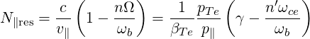
| Nb∥ | =  | (4.273) | |
| N∥res | =   | ||
=    | (4.274) |
where
| Ω | =  = =  with ωce = with ωce =  | (4.275) |
| n′ | = -n | (4.276) |
| βTe | =  = =  = =  | (4.277) |
The time-averaged energy flow density in the beam is in general given by
 | (4.278) |
where
![1- [ ^ ^*]
Pb = 2 Re Eb × H b](NoticeDKE2394x.png) | (4.279) |
is the flow of the electromagnetic energy or Poynting vector, and
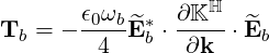 | (4.280) |
is the kinetic energy flow density where Kℍ is the Hermitian part of the dielectric tensor.
 b is the complex form of the electric field (4.250)
 | (4.281) |
and the magnetic field  b is given by
 | (4.282) |
using the relation Nb = kbωb∕c.
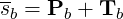
The energy flow density (4.278) can be formally rewritten as
 | (4.283) |
where Φb is a non dimensional vector defined as
 | (4.284) |
with
![[ ]
-μ0c-- ^ ^ *
ΦbP = |Eb0 |2Re Eb × H b](NoticeDKE2402x.png) | (4.285) |
and
 | (4.286) |
Using (4.282), we obtain
| ΦbP | = Re![[e × (N × e*)]
b b b](NoticeDKE2404x.png) | ||
= Re![*
[Nb - (Nb ⋅eb)eb]](NoticeDKE2405x.png) | (4.287) |
In vacuum, Φb =  , unit vector in the direction of propagation, and ΦbT = 0.
Here,
, unit vector in the direction of propagation, and ΦbT = 0.
Here,
 | (4.288) |
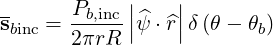
is the polarization vector. The incident power flux on a flux-surface is therefore given by
 | (4.289) |
where  is the local vector normal to the flux-surface.
The energy flows in the direction of the group velocity, noted 
 | (4.290) |
In ray-tracing calculations, this is the direction of the ray trajectories, which are parametrized
by  where s is the distance along the ray. Therefore
  b can be
determined from ray-tracing calculations or any other wave propagation model, and we
have
b can be
determined from ray-tracing calculations or any other wave propagation model, and we
have
 | (4.291) |
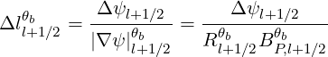
In DKE calculations, flux-surfaces are discretized on a grid ψl+1∕2 and have a finite volume
(). In consequence, the factor  must be ”integrated” along the ray trajectory within this
volume. We therefore define an incidence factor
must be ”integrated” along the ray trajectory within this
volume. We therefore define an incidence factor
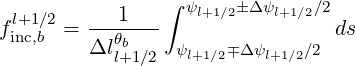 | (4.292) |
where the ± sign accounts for the fact that the ray may be locally directed either inward or outward, and where Δll+1∕2θb is the local thickness of the flux-surface.
 | (4.293) |
The factor finc,bl+1∕2 can be numerically calculated from the equilibrium and ray-tracing data. In the limit of an infinitely thin flux-surface, we have
 | (4.294) |
We therefore substitute
 | (4.295) |
Let consider a ray which crosses the flux surface at the respective poloidal locations θb. Here, it is assumed that all electrons interact with the beam, whatever its toroidal location, because of the axisymmetry. Therefore, calculations are only valid for circulating electrons, except for those localized on low n order rational q-surfaces, since their trajectories are exactly periodic in configuration space. Consequently, either they may never crosses the beam or if they cross it, the quasilinear assumption might likely fail, since some correlations could remain between two momentum kicks. However, the total weight of these electrons is marginal, and their contribution to RF power absorption and current generation is simply neglected. It is important to recal that trapped particle interaction with RF wave is not addressed in this code for similar arguments. For all particles whose trajectory is periodic, a specific treatment of the quasilinear interaction is necessary, which is at this stage beyond the scope of this development.
If we assume that the extension of the beam power on the flux-surface is very small in the poloidal directions, we can approximate
 | (4.296) |
This assumption is in contradication with the plane-wave decomposition of the RF beam,
since plane waves are essentially present in the entire configuration space. However, it is
assumed that plane waves interfere destructively everywhere except in the beam region, which
can be limited to a narrow poloidal and toroidal extention. By definition,  b is determined so
that Pb,inc is the total incident power on the flux-surface
b is determined so
that Pb,inc is the total incident power on the flux-surface
 | (4.297) |
which gives in the system  , using (A.199)
 | (4.298) |
Hence,
 | (4.299) |
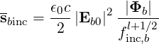
and the incident power flux is simply
 | (4.300) |
 | (4.301) |
For concentric circular flux surfaces,  =
=  , then
  = 1. We obtain
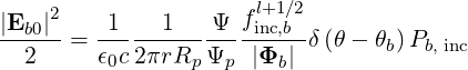 | (4.302) |
where Ψp = Ψp
= Ψp = 1 + ϵ.
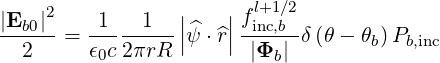
The diffusion coefficient is usually normalized to the collisional diffusion coefficient νepTe2, thus defining
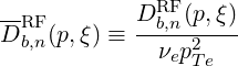 | (4.303) |
with
 | (4.304) |
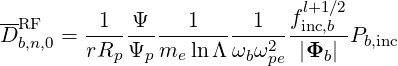
Using (4.271) and (4.301), the diffusion coefficient (4.303) becomes
 | (4.305) |
with
| Db,n,0RF | =        Pb,inc Pb,inc | ||
=      Pb,inc Pb,inc | (4.306) |
where ωpe is the electron plasma frequency
 | (4.307) |
We also recall the expressions (4.272), (4.274) and (4.284-4.287)
 | (4.308) |
 | (4.309) |
| Φb | = ΦbP + ΦbT | (4.310) |
| ΦbP | = Re![*
[Nb - (Nb ⋅eb)eb]](NoticeDKE2451x.png) | (4.311) |
| ΦbT | = - eb*⋅ eb*⋅ ⋅ eb ⋅ eb | (4.312) |
For concentric circular flux surfaces,
 | (4.313) |
In the Fokker-Planck equation, the diffusion and convection elements are bounce-averaged according to the expressions (3.189) and (3.194), which gives, using (4.233-4.236)
| DppRF(0) | =  | (4.314) | |
| DpξRF(0) | = σ![{ +∞ ∘ ------[ ] }
--σξ-- ∑ ∑ --1--ξ2- 2 nΩ- RF
√ Ψξ0 - ξ 1- ξ - ωb Db,n (p,ξ)
n=-∞ b](NoticeDKE2456x.png) | ||
| DξpRF(0) | = σ![{ ∘ ------[ ] }
--σξ-- +∑∞ ∑ --1--ξ2- 2 nΩ- RF
√ Ψξ - ξ 1- ξ - ω Db,n (p,ξ)
0 n=-∞ b b](NoticeDKE2457x.png) | ||
| DξξRF(0) | = ![{ }
ξ2 +∑∞ ∑ 1 [ nΩ ]2
--2- -2 1- ξ2 - --- DRFb,n(p,ξ)
Ψξ0 n=-∞ b ξ ωb](NoticeDKE2458x.png) |
where ()
![[ ]
1 1∑ ∫ θmax dθ 1 r B ξ0
{O } = λ^q- 2- 2π||----||R--B---ξ O
σ T θmin |^ψ ⋅^r| p P](NoticeDKE2459x.png) | (4.315) |
Since 1 - ξ2 = Ψ ,
,
| DppRF(0) | = ∑ n=-∞+∞∑ b(1 - ξ02)D b,nRF(0)(p,ξ 0) | (4.316) | |
| DpξRF(0) | = ∑
n=-∞+∞∑
b - ![[ 2 nΩ0 ]
1- ξ0 - -ω--
b](NoticeDKE2462x.png) Db,nRF(0)(p,ξ
0) Db,nRF(0)(p,ξ
0) | ||
| DξpRF(0) | = ∑
n=-∞+∞∑
b - ![[ ]
2 nΩ0-
1- ξ0 - ωb](NoticeDKE2464x.png) Db,nRF(0)(p,ξ
0) Db,nRF(0)(p,ξ
0) | ||
| DξξRF(0) | = ∑
n=-∞+∞∑
b ![[ nΩ ]
1- ξ20 - ---0
ωb](NoticeDKE2466x.png) 2D
b,nRF(0)(p,ξ
0) 2D
b,nRF(0)(p,ξ
0) |
where
 | (4.317) |
and Ω0 is the cyclotron frequency taken at the minimum B value, according to the relation
 | (4.318) |
with
 | (4.319) |
Therefore, only the bounce averaged diffusion coefficient Db,nRF(0)(p,ξ0) has to be calculated for the different types of RF waves, keeping the same formalism. It is determined by inserting expression (4.305) into (4.317),
 | (4.320) |
which gives
 | (4.321) |
We perform the poloidal integration
 | |||
=  ![[ ]
1∑
2
σ](NoticeDKE2474x.png) T ∫
θminθmax
dθ T ∫
θminθmax
dθ    ΨDb,n,0RF ΨDb,n,0RF 2δ 2δ δ δ | (4.322) | ||
=     ΨθbDb,n,0RF,θb
H ΨθbDb,n,0RF,θb
H H H ![[ ∑ ]
1-
2 σ](NoticeDKE2488x.png) T δ T δ  2 2 | (4.323) |
with
 θb θb | =  (ψ,θb) (ψ,θb) | (4.324) |
| rθb | = r | (4.325) |
| Rθb | = R | (4.326) |
| Bθb | = B | (4.327) |
| BP θb | = BP  | (4.328) |
| Ψθb | =  = =  | (4.329) |
| ξθb | = ξ = σ = σ | (4.330) |
and where H is the usual Heaviside step function
Therefore,
| Db,nRF(0)(p,ξ 0) | =      ΨθbDb,n,0RF,θb
× ΨθbDb,n,0RF,θb
× | ||
H H H ![[ ]
1-∑
2
σ](NoticeDKE2509x.png) T δ T δ  2 2 | (4.331) |
where we define, using (4.308), (4.309) and (4.306),
 | (4.332) |
 | (4.333) |
 | (4.334) |
with
| zbθb | =  | ||
= -Nb⊥   | |||
= -Nb⊥   | (4.335) |
In the Drift Kinetic equation, the diffusion and convection elements are bounce-averaged according to the expressions (3.218) and (3.223), which gives, using (4.233-4.236)
 ppRF(0) ppRF(0) | = σ | (4.336) | |
 pξRF(0) pξRF(0) | = ![{ ∘ ------ }
ξ2 +∑ ∞ ∑ 1- ξ2[ 2 n Ω] RF
-3∕2-2- - -------- 1 - ξ - --- D b,n(p,ξ)
Ψ ξ0n=- ∞ b ξ ωb](NoticeDKE2525x.png) | ||
 ξpRF(0) ξpRF(0) | = ![{ ξ2 +∑ ∞ ∑ ∘1----ξ2[ n Ω] }
-3∕2-2- - -------- 1 - ξ2 ---- DRFb,n(p,ξ)
Ψ ξ0n=- ∞ b ξ ωb](NoticeDKE2527x.png) | ||
 ξξRF(0) ξξRF(0) | = σ![{ 3 +∑∞ ∑ [ ]2 }
σ-ξ-- 1- 1 - ξ2 - nΩ- DRFb,n(p,ξ)
Ψ2ξ30 n=-∞ b ξ2 ωb](NoticeDKE2529x.png) |
and
 pRF(0) pRF(0) | =  ![{ }
(Ψ - 1) +∑∞ ∑ ∘1----ξ2[ nΩ ]
---3∕2- - -------- 1- ξ2 - --- DRFb,n(p,ξ)
Ψ n=-∞ b ξ ωb](NoticeDKE2532x.png) | (4.337) | |
 ξRF(0) ξRF(0) | =  σ σ![{ +∑∞ ∑ [ ]2 }
σξ(Ψ---1)- 1- 1 - ξ2 - n-Ω DRFb,n(p,ξ)
ξ0Ψ2 n=-∞ b ξ2 ωb](NoticeDKE2535x.png) |
where
![[ ]
1 1∑ ∫ θmax dθ 1 r B ξ
{O } = --- -- --|----|-------0O
λ^q 2 σ T θmin 2π||^ψ ⋅^r||Rp BP ξ](NoticeDKE2536x.png) | (4.338) |
Since 1 - ξ2 = Ψ and Ω = ΨΩ0,
 ppRF(0) ppRF(0) | = ∑
n=-∞+∞∑
b(1 - ξ02) b,nRF(0)D(p,ξ
0)
b,nRF(0)D(p,ξ
0) | (4.339) |
 pξRF(0) pξRF(0) | = ∑
n=-∞+∞∑
b - ![[ 2 nΩ0 ]
1- ξ0 - -ω--
b](NoticeDKE2542x.png)  b,nRF(0)D(p,ξ
0) b,nRF(0)D(p,ξ
0) | (4.340) |
 ξpRF(0) ξpRF(0) | = ∑
n=-∞+∞∑
b - ![[ ]
2 nΩ0-
1- ξ0 - ωb](NoticeDKE2546x.png)  b,nRF(0)D(p,ξ
0) b,nRF(0)D(p,ξ
0) | (4.341) |
 ξξRF(0) ξξRF(0) | = ∑
n=-∞+∞∑
b ![[ nΩ ]
1 - ξ20 - --0-
ωb](NoticeDKE2550x.png) 2 2 b,nRF(0)D(p,ξ
0)
b,nRF(0)D(p,ξ
0) | (4.342) |
 pRF(0) pRF(0) | =  ∑
n=-∞+∞∑
b - ∑
n=-∞+∞∑
b - ![[ ]
2 nΩ0-
1- ξ0 - ωb](NoticeDKE2555x.png)  b,nRF(0)F(p,ξ
0) b,nRF(0)F(p,ξ
0) | (4.343) | |
 ξRF(0) ξRF(0) | =  ∑
n=-∞+∞∑
b ∑
n=-∞+∞∑
b ![[ ]
1 - ξ20 - nΩ0-
ωb](NoticeDKE2560x.png) 2 2 b,nRF(0)F(p,ξ
0)
b,nRF(0)F(p,ξ
0) |
where
 b,nRF(0)D(p,ξ
0) b,nRF(0)D(p,ξ
0) | = σ | (4.344) | |
 b,nRF(0)F(p,ξ
0) b,nRF(0)F(p,ξ
0) | = σ |
and Ω0 is the cyclotron frequency taken at the minumum B value, as defined
for the Fokker-Planck equation. Therefore, only the two bounce averaged diffusion
coefficient  b,nRF(0))D(p,ξ0) and
  b,nRF(0)F(p,ξ0) have to be calculated for the different
types of RF waves, keeping also the same formalism. It is important to recall that
only
b,nRF(0)F(p,ξ0) have to be calculated for the different
types of RF waves, keeping also the same formalism. It is important to recall that
only  = σξ0 can be put outside the
  corresponding of the bounce-averaging
integral.
corresponding of the bounce-averaging
integral.
These coefficient are determined by inserting expression (4.305) into (4.317),
 b,nRF(0)D(p,ξ
0) b,nRF(0)D(p,ξ
0) | = σ | (4.345) | |
 b,nRF(0)F(p,ξ
0) b,nRF(0)F(p,ξ
0) | = σ |
which gives
 b,nRF(0)D(p,ξ
0) b,nRF(0)D(p,ξ
0) | =  σ σ | (4.346) | |
 b,nRF(0)F(p,ξ
0) b,nRF(0)F(p,ξ
0) | =  σ σ |
We perform the poloidal integration
σ | |||
=  σ σ![[ ]
1-∑
2
σ](NoticeDKE2582x.png) T ∫
θminθmax
dθ T ∫
θminθmax
dθ    σDb,n,0RF σDb,n,0RF 2δ 2δ δ δ | |||
=     Db,n,0RF,θb
H Db,n,0RF,θb
H H H σ σ![[ ]
1 ∑
--
2 σ](NoticeDKE2596x.png) T σδ T σδ  2 2 | (4.347) |
σ | |||
=  σ σ![[ ∑ ]
1-
2 σ](NoticeDKE2601x.png) T ∫
θminθmax
dθ T ∫
θminθmax
dθ     σDb,n,0RF σDb,n,0RF | |||
× 2δ 2δ δ δ | |||
=      Db,n,0RF,θb
H Db,n,0RF,θb
H H H | |||
× σ![[ ]
1∑
2
σ](NoticeDKE2617x.png) T σδ T σδ  2 2 | (4.348) |
where H is the usual Heaviside step function and Db,n,0RF,θb is given by (4.331).
Therefore, we find
 b,nRF(0)D(p,ξ
0) b,nRF(0)D(p,ξ
0) | =      Db,n,0RF,θb
× Db,n,0RF,θb
× | (4.349) | |
H H H σ σ![[ ∑ ]
1-
2 σ](NoticeDKE2629x.png) T σδ T σδ  2 2 |
 b,nRF(0)F(p,ξ
0) b,nRF(0)F(p,ξ
0) | =       Db,n,0RF,θb
× Db,n,0RF,θb
× | (4.350) | |
H H H σ σ![[ ]
1-∑
2
σ](NoticeDKE2641x.png) T σδ T σδ  2 2 |
The quasilinear diffusion coefficients (4.331), (4.349) and (4.350) describe the interaction
between electrons and a discrete set (b) of RF plane waves (4.250) with frequencies ωb. In
addition, we can linearly superpose a discrete set of plane waves with the same frequency but
different parallel wave number k∥ because of the linearity of the QL operator (4.188) in k. This
set of plane waves is typically represented by rays. Each ray is characterized by: the wave
frequency ωb, the poloidal location θb, the index of refraction Nb, the polarization vector eb and
the power flow Φb. In general, the ray propagation path  and the evolution of the index of
refraction Nb are determined by ray-tracing (RT) calculations. When the wave properties are
determined by RT calculations, the launched power spectrum in k∥ is typically decomposed in
an array of rays with different poloidal launching angle and/or k∥ power spectrum. This
distribution depends on the antenna and other launching parameters. The evolution of each
ray is determined separately, by the RT code, and the contributions of each ray to
wave-particle interaction are separately accounted for in the sum over b in (4.233-4.236).
The separation of these contributions is justified if their k∥ power spectrums do not
overlap.
and the evolution of the index of
refraction Nb are determined by ray-tracing (RT) calculations. When the wave properties are
determined by RT calculations, the launched power spectrum in k∥ is typically decomposed in
an array of rays with different poloidal launching angle and/or k∥ power spectrum. This
distribution depends on the antenna and other launching parameters. The evolution of each
ray is determined separately, by the RT code, and the contributions of each ray to
wave-particle interaction are separately accounted for in the sum over b in (4.233-4.236).
The separation of these contributions is justified if their k∥ power spectrums do not
overlap.
We do not address the RT problem in this work. Therefore, we assume that the path θb and the parallel index of refraction Nb∥ are determined either by coupling of DKE to a RT code,
or by any other propagation model. RT calculations require to calculate the dispersion tensor
and solve the dispersion relation, and therefore they can provide input for the remaining wave
properties
and the parallel index of refraction Nb∥ are determined either by coupling of DKE to a RT code,
or by any other propagation model. RT calculations require to calculate the dispersion tensor
and solve the dispersion relation, and therefore they can provide input for the remaining wave
properties  . However, these properties can also be determined by solving locally the
wave equation, once ψ,θb and N∥ are known. Keeping the calculation of
. However, these properties can also be determined by solving locally the
wave equation, once ψ,θb and N∥ are known. Keeping the calculation of  within
DKE allows us to use a more advanced model - such as the fully relativistic dispersion solver
R2D2 - for the evaluation of these important wave properties. A numerical code is
required to solve the wave equation, and evaluate the diffusion coefficient (4.331) in the
general case. However, it is possible to obtain analytic expressions in some cases,
assuming that the waves can be treated in the cold plasma limit. The calculation of
Db,nRF(0)(p,ξ0) in the cold plasma model is performed in Appendix D. In addition,
simplified expression and the comparison with operators used in the litterature are given
for lower-hybrid (LH) and electron-cyclotron (EC) waves in appendices D.2 and D.3
respectively.
within
DKE allows us to use a more advanced model - such as the fully relativistic dispersion solver
R2D2 - for the evaluation of these important wave properties. A numerical code is
required to solve the wave equation, and evaluate the diffusion coefficient (4.331) in the
general case. However, it is possible to obtain analytic expressions in some cases,
assuming that the waves can be treated in the cold plasma limit. The calculation of
Db,nRF(0)(p,ξ0) in the cold plasma model is performed in Appendix D. In addition,
simplified expression and the comparison with operators used in the litterature are given
for lower-hybrid (LH) and electron-cyclotron (EC) waves in appendices D.2 and D.3
respectively.
Note that the cold plasma model, if used in the RT calculations, does not account for the wave-particle interaction and the power absorption from the rays. The power absorbed from each ray and deposited on electrons can be evaluated if a hot plasma model is used, but even then, the calculation is not consistent with DKE because quasilinear effects are not accounted for. In order to have a consistency between RT and DKE calculations, the power absorption calculated by DKE must be inserted back in the RT calculations. In the case where rays turn back toward the edge (as it can happen in LHCD), iterations between RT and DKE calculations are necessary to ensure self-consistency.
We consider two different models for the k∥ spectrum of a given ray.
Square power spectrum in k∥ Here, the power spectrum of a given ray is taken as being constant in N∥ between two limits Nb∥ min and Nb∥ max. Therefore, we operate the following transformation
 | (4.351) |
where
 | (4.352) |
In this case, the RT calculations and wave equation are solved for the central value.
 | (4.353) |
which is a good approximation only when
 | (4.354) |
For simplification and benchmarking purposes, in LHCD, one can consider only one ray with a square spectrum. Then, the limits Nb∥ min and Nb∥ max are respectively given by the accessibility condition and the condition for strong linear Laudau damping.
Gaussian power spectrum in k∥ The power spectrum of a given ray can be assumed to have a Gaussian dependence on N∥, centered around a value Nb∥,0 and with a Gaussian width ΔNb∥. Then, we operate the transformation
![[ ( )2 ]
δ (N - N ) → √---1----exp ---N∥res --Nb∥,0-
b∥ ∥res πΔNb ∥ ΔN 2b∥](NoticeDKE2652x.png) | (4.355) |
In this case too, the RT calculations and wave equation are solved for the central value Nb∥,0, which is a good approximation only when
 | (4.356) |
For simplification and benchmarking purposes, in ECCD, one can consider only one ray with a Gaussian spectrum. Then, the wave properties Nb∥,0 and ΔNb∥ are determined by the beam characteristics, as described in 4.3.9.
If we consider a Gaussian beam of waist d, of negligible diffraction angle, and of negligible dispersion, such that the wave vector is in the direction of the beam, and N ≃ 1, we get that by the properties of Fourier transform, the width ΔN∥ is related to the beam waist d as
 | (4.357) |
This conditions are approximately satisfied for EC beamsif the density is low (ωpe ≪ ω).
Then, and we can verify that for a beam waist of a few centimeters (d = 5 cm, f = 110 GHz, N∥≃ 0.2 → ΔN∥≃ 0.01), the condition (4.356) is satisfied, and there is no nead to decompose the beam spectrum into many rays.