5.6 Initial solution

5.6.1 Zero order term: the Fokker-Planck equation

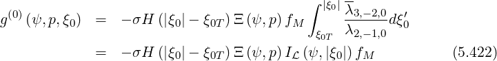
Basically, the determination of the steady-state electron distribution function is an initial value problem, where the initial guess corresponds usually to the unperturbed solution of the linearized problem. For the zero-order Fokker-Planck equation, the Maxwellian distribution function is therefore by definition an eigenfunction of the collision operator, without external perturbation. Here the weakly relativistic solution corresponding to the condition on the relativistic factor γ - 1 ≪ 1 is considered at time t = 0,

(5.398)

where T_e and n_e are the electron temperature and density respectively. Details on the notation are given in Sec. 6.3.1. Projected on the numerical grids, as defined in Sec.5.2, the discrete form is

(5.399)

When the Lower Hybrid current drive problem is addressed, it is possible to start from a guess that already incorporate the existence of a plateau region, using the formulation given in Ref. [?] in the non-relativistic limit. When relativistic corrections must be considered, the effective perpendicular temperature T_⊥ in the resonance domain must be usualy multipled by 2. Though this elegant approach seems attractive in order to reduce the total number of iterations for reaching the steady-state solution, its effectiveness is usualy poor when large time step Δt are considered. Indeed, the total number of time steps is merely determined by the relaxation time of the most energetic part of the fast electron tail prodiced by the wave. Since electrons are very weakly collisional, their relaxation time is very long as compared to the thermal one. Therefore, the gain for the rate of convergence is usually very small since the distribution model does not describe accurately the region above the plateau of the momentum space. Consequently, even if this method is implemented in the code, it is almost never used.

5.6.2 Up to first order term: the Drift Kinetic equation

First order distribution function The initial distribution function for the first order drift kinetic equation is determined in the non-relativistic limit using the simplified Lorentz collision model corresponding to Z_i ≫ 1 and T_i = 0, as introduced in Sec. 4.1.6. In that case, the bounce-averaged collision operator reduces to

(5.400)

and in the steady-state regime = 0 , so that the equation to be solved is simply

(5.401)

where

(5.402)

and

(5.403)

as defined in Sec.3.5.5.

Since only pitch-angle scattering takes place in this limit, _ξ0,⁽⁰⁾ may be expressed in a very simple form

(5.404)

since F_ξ^C = D_ξp^C = 0 for collisions with

(5.405)

while

(5.406)

with

(5.407)

where D_ξξ,^C = B_t according usual notation given in Sec.4.1.6.

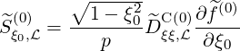
The differential equation to be solved is then

(5.408)

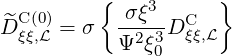
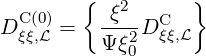
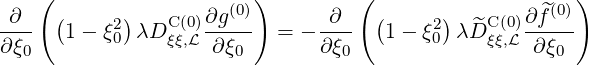
starting from the known expression of ∂ ⁽⁰⁾∕∂ξ₀. In the Lorentz limit, since B_t is simply set to 1∕2, expressions of D_ξξ,^C(0) and _ξξ,^C(0) are obtained in a straightforward manner,

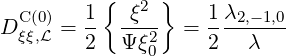(5.409)

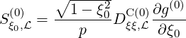
and

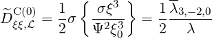(5.410)

and g⁽⁰⁾ is given by the simple equation

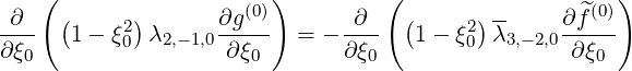(5.411)

If the solution of the zero-order Fokker-Planck equation is the Maxwellian

(5.412)

its spatial derivative is

(5.413)

and from the definition of ⁽⁰⁾ given in Sec.3.4,

Projected on the numerical grids, the discrete form of ⁽⁰⁾ is

Since f_M is by definition independent of ξ₀,

(5.417)

the equation becomes

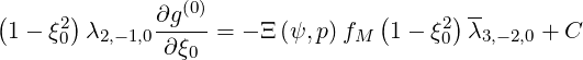(5.418)

Assuming ∂g⁽⁰⁾∕∂ξ₀ is finite at = 1, C = 0, and

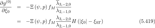
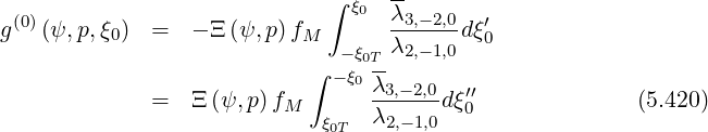
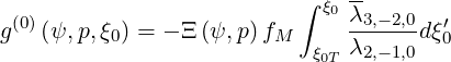(5.421)

and gathering results

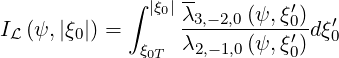(5.423)

The discrete form of g⁽⁰⁾ is

gl+1∕2,i+1∕2,j+1∕2(0)	= -σ j+1∕2H
	× Ξl+1∕2,i+1∕2IfM,l+1∕2,i+1∕2,j+1∕2	(5.424)

with

(5.425)

and j > j_T,l+1∕2⁺.

Case of circular concentric flux surfaces According to Sec. 4.1.7,

(5.426)

and Sec. 4.1.6

(5.427)

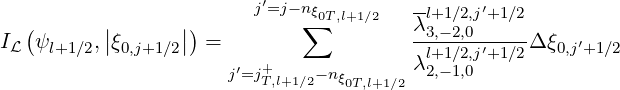
The integral I then becomes

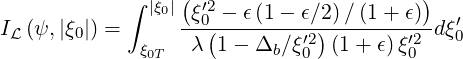(5.428)

and in the low inverse aspect ratio limit ϵ ≪ 1, one finds

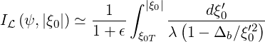(5.429)

the expression that was first given in Ref. [?].

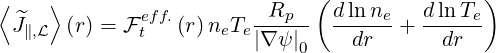
Flux surface averaged bootstrap current According to Sec. 3.6, the flux-averaged electron bootstrap current in the Lorentz model is given by the relation

(5.430)

where

(5.431)

and

(5.432)

in the non-relativistic limit γ → 1. Therefore,

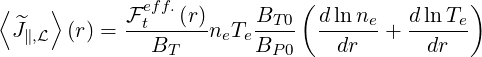
Using relation R₀B_T0 = I, one obtains

Since

(5.437)

using the definite integral relation in Ref. [?],

(5.438)

where !! = 1.3.5... ×,

Finally,

(5.441)

where the flux surface function usualy named “effective trapped fraction” _t^eff. is

In the case of circular concentric flux surfaces,

(5.443)

(5.444)

and

(5.445)

as shown in Sec. 3.6. Therefore,

(5.446)

and using the relations R₀B_P0 = ₀, and R₀B_T0 = I,

(5.447)

where R_pB_T = I. Hence,

	teff. = 2
		(5.448)

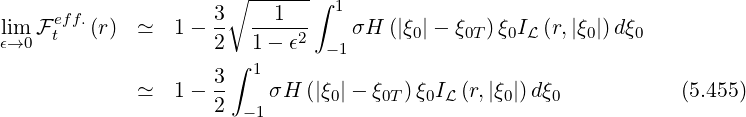
and since R₀∕R = Ψ, λ_2,-2,2 = λ_2,0,0, as shown in Sec. 3.6. In the limit B_p ≪ B_T , further simplifications may be carried out and

(5.449)

The first term in the square bracket may be evaluated analyticaly. Indeed

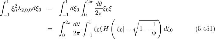
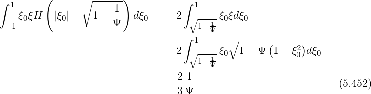
Consequently,

(5.454)

and using the

It can be shown in Appendix C after lengthly calculations, that

(5.456)

where

(5.457)

with

(5.458)

A rather fast convergence is obtained with m, and for m = n = 6, K ≃ 1.467, the usual value found in the litterature on neoclassical theory.