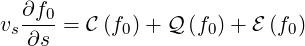
The Fokker-Planck Equation is
|
| (3.103) |
In the low collision regime, which is characterized by the condition
 | (3.104) |
where τdt = ϵτc is the collision detrapping time, as defined in the previous section, it is assumed that electrons circulating or trapped are able to complete their orbit in a time too short for collisions to deflect them from their orbit. As a consequence, the dominant term in the Fokker-Planck equation is simply
 | (3.105) |
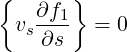
so that f0 is constant along the field lines.
Then, performing a bounce-averaging, we have
 | =  ![[ ]
1∑
2-
σ](NoticeDKE333x.png) T ∫
sminsmax T ∫
sminsmax
 vs vs | ||
=  ![[ ]
1∑
--
2 σ](NoticeDKE337x.png) T σ T σ![[f0]](NoticeDKE338x.png) sminsmax sminsmax
| (3.106) |
For passing particles, the positions smin and smax coincide, so that ![[f ]
0](NoticeDKE339x.png) sminsmax = 0 and the
term vanishes. For trapped particles, the term also vanishes because of the sum over σ = ±1,
since, by definition, v∥ = 0 at the turning points smin and smax, and consequently f0 is
independent of the sign of σ.
sminsmax = 0 and the
term vanishes. For trapped particles, the term also vanishes because of the sum over σ = ±1,
since, by definition, v∥ = 0 at the turning points smin and smax, and consequently f0 is
independent of the sign of σ.
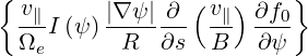
Therefore, the bounce-averaged Fokker-Planck equation becomes
 | (3.107) |
with f0 constant along the field lines.
The drift kinetic equation is
 | (3.108) |
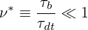
In the low collisiona regime ν*≪ 1, the dominant term is
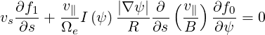 | (3.109) |
which gives
 | (3.110) |
where
 | (3.111) |
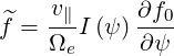
and g is a constant function along the field lines. Noting that
 | (3.112) |
we get
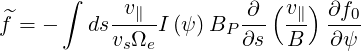
 | = ∫
ds I I B B   | ||
=   ∫
ds ∫
ds  | |||
=  I I  | (3.113) |
where we used the fact that ∂f0∕∂s = 0.
Then, performing a bounce-averaging, we find again, using the same argument as in (3.106), that
 | (3.114) |
In addition, we have
 | |||
=  ![[ ∑ ]
1-
2 σ](NoticeDKE362x.png) T ∫
sminsmax T ∫
sminsmax
  I I     | |||
=    ![[ ∑ ]
1-
2 σ](NoticeDKE373x.png) T σ ∫
sminsmax
ds T σ ∫
sminsmax
ds  | |||
=    ![[ ∑ ]
1-
2 σ](NoticeDKE379x.png) T σ T σ![[ ]
v∥
B](NoticeDKE380x.png) sminsmax sminsmax
| (3.115) |
Again, for passing particles, the positions smin and smax coincide, so that ![[ ]
v∥∕B](NoticeDKE381x.png) sminsmax = 0
and the term vanishes. For trapped particles, the term also vanishes because v∥→ 0 at the
turning points smin and smax.
sminsmax = 0
and the term vanishes. For trapped particles, the term also vanishes because v∥→ 0 at the
turning points smin and smax.
Consequently, we find that the bounce-averaged drift kinetic equation becomes
 | (3.116) |
where .
 | (3.117) |
 | (3.118) |
and g is then given by
 | (3.119) |
using the fact that all operators are linear.