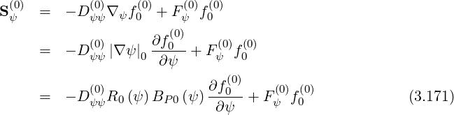
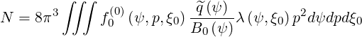
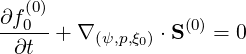
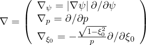
The starting point of the flux conservative representation is the conservation of the total number of particles in the plasma,
|
| (3.120) |
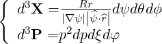
where X and P are respectively coordinates in configuration and momentum spaces. According
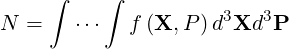
to the systems which are used in the calculations, X = and P =
 ,
,
 | (3.121) |
as shown in Appendix A, one obtains
 | (3.122) |
Using the transformation
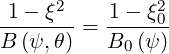 | (3.123) |
that results from conservation of the magnetic moment and energy,
 | (3.124) |
because ξdξ∕B = ξ0dξ0∕B0
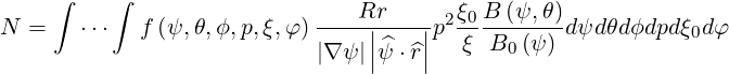
 . Since at the zero order, f0 is constant along a magnetic
field line, f0 = f0
. Since at the zero order, f0 is constant along a magnetic
field line, f0 = f0 is independent of the poloidal angle θ, where f0
 is the bounce averaged
distribution function. Hence
is the bounce averaged
distribution function. Hence
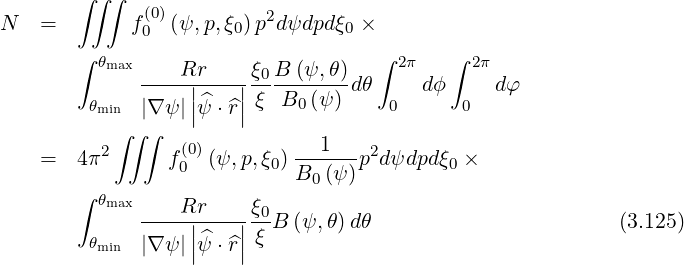
From plasma equilibrium, since
 | (3.126) |
where BP is the poloidal magnetic field,
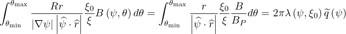 | (3.127) |
Here, appears, as expected the normalized bounce time λ and the factor
 introduced in Sec. 2.2.1, which in conjunction with B0
 characterizes the local shape of
magnetic flux surface. Hence,
characterizes the local shape of
magnetic flux surface. Hence,
 | (3.128) |
From this expression, the Jacobian J of the coordinate system  may be simply
defined as,
may be simply
defined as,
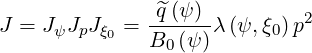 | (3.129) |
where
 | (3.130) |
and the generic conservative form of the kinetic equation may be immediatly deduced
 | (3.131) |
where the phase space flux S at B = Bmin is decomposed into a diffusive and a convective
part
at B = Bmin is decomposed into a diffusive and a convective
part
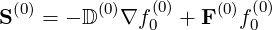 | (3.132) |
in the mean field theory. Here, D and F
and F are respectively the diffusion tensor and convection
vector in phase space. They can be expressed generally as
are respectively the diffusion tensor and convection
vector in phase space. They can be expressed generally as
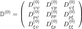 | (3.133) |
and
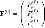 | (3.134) |
where each element is function of  . Here the gradient vector in the reduced
  space is
 | (3.135) |
so, following calculations given in Appendix A,
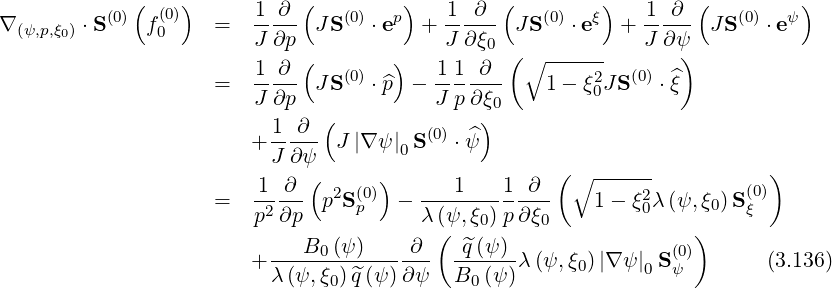
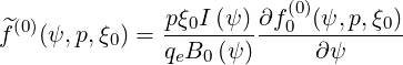
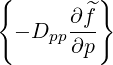
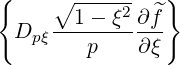
 0 is taken on the magnetic flux surface where B is minimum, i.e., B = B0. The first
two terms correspond to the usual dynamics in momentum space at a given spatial position ψ,
while the third one is associated to spatial transport at fixed p and ξ0. It is interesting to note
that spatial transport is not independent of the momentum dynamics through the parameter
λ
0 is taken on the magnetic flux surface where B is minimum, i.e., B = B0. The first
two terms correspond to the usual dynamics in momentum space at a given spatial position ψ,
while the third one is associated to spatial transport at fixed p and ξ0. It is interesting to note
that spatial transport is not independent of the momentum dynamics through the parameter
λ . It corrects the spatial transport from the particle dynamics along the magnetic field
line, since most particles tend to spend more time far from B = B0. In the limit of
strongly passing particles, λ
. It corrects the spatial transport from the particle dynamics along the magnetic field
line, since most particles tend to spend more time far from B = B0. In the limit of
strongly passing particles, λ ≃ 1, and the spatial term becomes independent of
ξ0.
≃ 1, and the spatial term becomes independent of
ξ0.
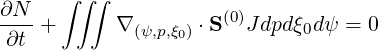
It is interesting to cross-check the conservative nature of the transport equation is well ensured by performing the integral
![[ ]
∫∫ ∫ ∂f(00) (0)
-∂t--+ ∇ (ψ,p,ξ0) ⋅S Jdpd ξ0dψ = 0](NoticeDKE422x.png) | (3.137) |
or
 | (3.138) |
Indeed, in that case, the variation of the total number of particles ∂N∕∂t as a function of time depends only from boundary conditions.
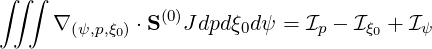 | (3.139) |
where
 | (3.140) |
 | (3.141) |
 | (3.142) |
For  p,
p,
![∫ ∫∫
1--∂-( 2 (0))
p2∂p p S p J dpdξ0dψ
∫ ∫ [ ]pmax
= p2S(p0) q^(ψ)-λ(ψ, ξ0) dξ0d ψ
∫∫ 0 B0 (ψ )
2 (0) -^q(ψ)-
= pmax Sp (pmax) B0 (ψ )λ (ψ, ξ0)dξ0dψ (3.143)](NoticeDKE428x.png)
 = 0, one finds p = 0. This condition is generally well
fullfiled, except in strong runaway regimes, where above the Dreicer limit characterized
by critical momentum pD, electrons gain energy up to very high energies, that are
usually well beyond the domain of integration addressed in numerical calculations
for the current drive problem. However, in this case, p is given by Sp
= 0, one finds p = 0. This condition is generally well
fullfiled, except in strong runaway regimes, where above the Dreicer limit characterized
by critical momentum pD, electrons gain energy up to very high energies, that are
usually well beyond the domain of integration addressed in numerical calculations
for the current drive problem. However, in this case, p is given by Sp at pmax,
where pmax corresponds to the boundary of the momentum domain of integration. Its
conservative nature is well ensured, since ∂N∕∂t only depends of this parameter for
p.
at pmax,
where pmax corresponds to the boundary of the momentum domain of integration. Its
conservative nature is well ensured, since ∂N∕∂t only depends of this parameter for
p.
The integration of ξ0 leads to
![∫∫ ∫ ( ∘ ------ )
---1----1-∂--- 2 (0)
Iξ0 = λ (ψ,ξ0)p ∂ξ0 1- ξ0λ (ψ,ξ0)Sξ J dpdξ0dψ
∫∫ [∘ ------ ]+1
= 1- ξ2λ (ψ,ξ0)S(0) -^q(ψ-)pdpd ψ
0 ξ -1B0 (ψ)
= 0 (3.144)](NoticeDKE431x.png)
Finally,
![∫ ∫∫ B0 (ψ) ∂ ( ^q (ψ ) (0))
Iψ = λ(ψ,-ξ)-^q(ψ)∂-ψ B--(ψ-)λ(ψ,ξ0)|∇ ψ|Sψ J dpdξ0dψ
∫ ∫ [ 0 0 ]ψ
-^q-(ψ-)-- (0) a 2
= Bmin(ψ )λ(ψ,ξ0)|∇ ψ|Sψ 0 p dpdξ0
q^(ψ ) ∫∫
= ----a--|∇ψ |ψa λ(ψa,ξ0)S(ψ0)(ψa)p2dpdξ0 (3.145)
B0 (ψa )](NoticeDKE432x.png)
 0 = R0BP0 = 0 at ψ = 0 when no particle is
injected at the plasma center. Here, BP0 is the poloidal magnetic field where B is
minimum. If Sψ
0 = R0BP0 = 0 at ψ = 0 when no particle is
injected at the plasma center. Here, BP0 is the poloidal magnetic field where B is
minimum. If Sψ
 = 0, ψ = 0, and the total number of particles is conserved in the
discharge.
= 0, ψ = 0, and the total number of particles is conserved in the
discharge.
It is important to notice that the magnetic moment is intrinsically conserved in the equations, in particular for the radial transport part, through the pitch-angle dependence of the normalized bounce time λ. Therefore, spatial transport is valid not only for circulating particles satisfying p∥∕p⊥≫ 1, but also for highly trapped electrons, i.e. when p∥∕p⊥≪ 1.
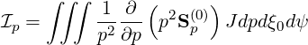
Momentum space operator It is possible to recover the general bounce averaged transport equation in momentum space by another independent approach. Here, the momentum space dynamics of the kinetic equation is be expressed in conservative form as a flux divergence that may expressed according to the (A.57) introduced in Appendix A
 | (3.146) |
where Jp is the momentum space Jacobian associated with the momentum space coordinate
system  , described in (A.247). Since the spherical system has the natural symmetry of
collisions, the momentum space Jacobian is (A.269)
, described in (A.247). Since the spherical system has the natural symmetry of
collisions, the momentum space Jacobian is (A.269)
 | (3.147) |
so that, taking into account that the kinetic equation is gyroaveraged and therefore the coordinate φ disappears, the following expression for the divergence (A.278) is obtained
 | (3.148) |
where by definition
| Sp | = Sp ⋅ | (3.149) |
| Sξ | = Sp ⋅ | (3.150) |
In the mean-field theory, the momentum space fluxes may be expressed as the sum of diffusive and convective parts,
 | (3.151) |
with
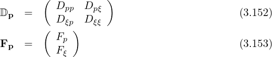
The gradient vector ∇p in the reduced coordinates system  in given by (A.277)
 | (3.154) |
with
| ∇p | =  | (3.155) |
| ∇ξ | = -  | (3.156) |
so that
 | (3.157) |
and
 | (3.158) |
Bounce-averaged operator The bounce averaged operator is
 | (3.159) |
where the bounce averaging operation is defined in (2.62)
![[ ∑ ] ∫ θmax
{A } = 1-- 1- dθ|-1--|-r--B-ξ0A
λ^q 2 σ T θmin 2π||^ψ ⋅^r||Rp BP ξ](NoticeDKE452x.png) | (3.160) |
and ξ is given along the trajectory by
 | (3.161) |
with
 | (3.162) |
as shown in Sec.2.2.1.
We find from (3.161) that in momentum space
 | (3.163) |
and we also get
 | (3.164) |
Then, keeping in mind that  = σξ0 is independent of σ, we can transform as
follows,
= σξ0 is independent of σ, we can transform as
follows,
 | |||
=  ![[ ∑ ]
1-
2 σ](NoticeDKE460x.png) T ∫
θminθmax T ∫
θminθmax
        | |||
=    ![[ ]
1-∑
2
σ](NoticeDKE472x.png) T ∫
θminθmax T ∫
θminθmax
      | |||
=    σ σ ![[ ∑ ]
1-
2 σ](NoticeDKE483x.png) T ∫
θminθmax T ∫
θminθmax
      | |||
=    λσ λσ | (3.165) |
using relation ξdξ = Ψξ0dξ0 that is deduced from expression (3.161).
Finally, we can rewrite the equation (3.159) in a conservative form as
 | (3.166) |
where the following components are defined
 | (3.167) |
and
 | (3.168) |
Here, expression (3.166) is completely equivalent to the momentum transport equation deduced from particle conservation. However, this equivalence may be used only because the bounce-averaged operator is local, and does not depends of ψ.
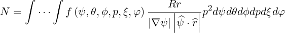
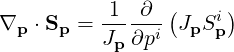
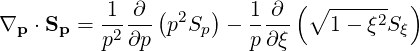
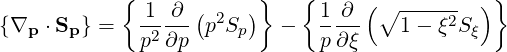
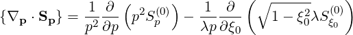
Configuration space operator The operator that describes the spatial transport is given by relation
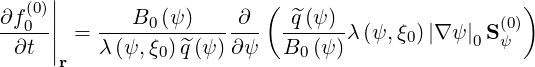 | (3.169) |
and since BP =  ∕R, it may be rewritten in the form
 | (3.170) |
where R0 and BP0 are taken at the poloidal location where the magnetic field is minimum B = B0. Much in the same way,
where the diffusion cross-terms Dpψ , Dψp
, Dψp ,Dξψ
,Dξψ and Dψξ
 between momentum and
configuration spaces have been neglected.
between momentum and
configuration spaces have been neglected.
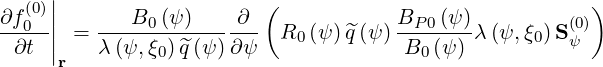
Case of circular concentric flux-surfaces
In that case,  =
=  , and by definition Dψψ
 = Drr
= Drr , Fψ
, Fψ = Fr
= Fr , since ψ is here just a
label. Therefore, using relation
, since ψ is here just a
label. Therefore, using relation  0∂∕∂ψ = ∂∕∂r,
Furthermore, since
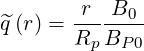 | (3.173) |
one obtains,
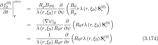
Note that R0 may not be here simplified, since it is a function of r, which corresponds to the
toroidal configuration. Dynamics in momentum and configuration spaces are also not decoupled,
the normalized bounce time λ being on both sides of the radial derivative. Only for
strongly circulating electrons,
being on both sides of the radial derivative. Only for
strongly circulating electrons,
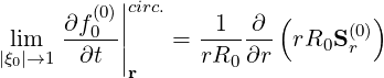 | (3.175) |
since lim →1λ
→1λ = 1, and the usual cylindrical conservative expression of the radial
transport
= 1, and the usual cylindrical conservative expression of the radial
transport
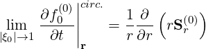 | (3.176) |
is only found in the case ϵ ≪ 1, i.e. when R0 ≈ Rp.
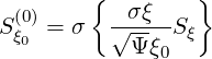
The bounce averaged Fokker-Planck equation is is given in the conservative form by relation (3.166), with the bounce-averaged fluxes (3.167) and (3.168)
Sp | =  | (3.177) |
Sξ0 | = σ | (3.178) |
Because f0 is constant along a magnetic field line, we have f0 = f0(0)
 which is
independent of θ and σ. Using the following identities
which is
independent of θ and σ. Using the following identities
- | = -  | (3.179) |
 | =    | (3.180) |
 | =  f0(0) f0(0) | (3.181) |
- σ | = -σ  | (3.182) |
σ | =  σ σ  | (3.183) |
σ | = σ f0(0) f0(0) | (3.184) |
we can rewrite
 | (3.185) |
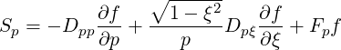
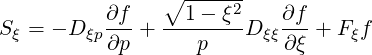
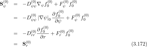
where the bounce averaged flux is decomposed into
 | (3.186) |
with
| Sp(0) | = -D
pp(0) + +  Dpξ(0) Dpξ(0) + Fp(0)f
0(0) + Fp(0)f
0(0) | (3.187) |
| Sξ0(0) | = -D
ξp(0) + +  Dξξ(0) Dξξ(0) + Fξ(0)f
0(0) + Fξ(0)f
0(0) | (3.188) |
by defining the diffusion components
| Dpp(0) | =  | (3.189) |
| Dpξ(0) | = σ | (3.190) |
| Dξp(0) | = σ | (3.191) |
| Dξξ(0) | =  | (3.192) |
and the convection components
| Fp(0) | =  | (3.193) |
| Fξ(0) | = σ | (3.194) |
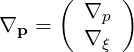
where the gradient vector in the reduced  momentum space is
 | (3.195) |
with
| ∇p | =  | (3.196) |
| ∇ξ0 | =   | (3.197) |
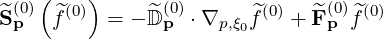
In the first-order drift kinetic equation, the momentum space operator
 | (3.198) |
where the fluxes are expressed as (3.151) may be decomposed as
 | (3.199) |
According to (3.166), we can express the bounce-averaged operator as
 | =   - -   | (3.200) |
 | =   - -   | (3.201) |
where we need to evaluate the bounce-averaged fluxes (3.167) and (3.168) for  and g
respectively
and g
respectively
 p p | =  | (3.202) |
 ξ0 ξ0 | = σ | (3.203) |
and
Sp | =  | (3.204) |
Sξ0 | = σ | (3.205) |
Because g is constant along a field line, we have g = g(0)
 which is independent of θ
and σ. Therefore, the fluxes for g have exactly the same expression as for f0 in the zero-order
equation described in section. This is why the same notation in (3.201) is used, while the fluxes
associated with
which is independent of θ
and σ. Therefore, the fluxes for g have exactly the same expression as for f0 in the zero-order
equation described in section. This is why the same notation in (3.201) is used, while the fluxes
associated with  are noted
  .
.
Indeed,  has an explicit dependence upon θ, which can be isolated as follows:
 | (3.206) |
with
 | (3.207) |
We can note that  (0) is antisymmetric in the trapped region, since f0(0) is symmetric and ξ0
is, of course, antisymmetric. As a result, only σ
(0) is antisymmetric in the trapped region, since f0(0) is symmetric and ξ0
is, of course, antisymmetric. As a result, only σ (0) can be taken out of the bounce averaging
operator. Taking the bounce-average of each term, we find
(0) can be taken out of the bounce averaging
operator. Taking the bounce-average of each term, we find
 | = -σ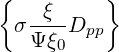  | (3.208) | |
 | =    | ||
+  σ σ  (0) (0) | (3.209) | ||
 | = σ  (0) (0) | (3.210) | |
- σ | = -  | (3.211) | |
σ | =  σ σ  | ||
+    (0) (0) | (3.212) | ||
σ | =   (0) (0) | (3.213) |
where the following relation is used
  | = σ  | ||
= σ | |||
= σ | (3.214) |
We can therefore rewrite
where the bounce averaged flux is decomposed into
 | (3.215) |
with
 p(0) p(0) | = - pp(0)
pp(0) + +   pξ(0) pξ(0) + +  p(0) p(0) (0) (0) | (3.216) |
 ξ0(0) ξ0(0) | = - ξp(0)
ξp(0) + +   ξξ(0) ξξ(0) + +  ξ(0) ξ(0) (0) (0) | (3.217) |
by defining the diffusion components
 pp(0) pp(0) | = σ | (3.218) |
 pξ(0) pξ(0) | =  | (3.219) |
 ξp(0) ξp(0) | =  | (3.220) |
 ξξ(0) ξξ(0) | = σ | (3.221) |
and the convection components
 p(0) p(0) | = σ + +   | (3.222) |
 ξ(0) ξ(0) | =  + +  σ σ | (3.223) |
where we use the fact that σξ03 may be taken out of the bounce averaged operator, since ξ03
is an odd function of ξ0. The gradient vector in the reduced  momentum space
is
momentum space
is
 | (3.224) |
with
| ∇p | =  | (3.225) |
| ∇ξ0 | =   | (3.226) |