6.1 Matrix representation

6.1.1 Zero order term: the Fokker-Planck equation

Implicit time scheme

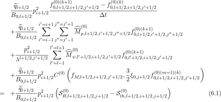
Projected on the numerical distribution function grid, and taking into account of the internal and external boundaries, the 3 - D electron Fokker-Planck equation may be expressed as

Upwind differencing corresponding to the fully implicit time scheme is used, since it is usually numerically stable for arbitrary values of Δt. Therefore, with this method, a fast rate of convergence towards the steady-state solution lim_k→∞f_{0,l+1∕2,i+1∕2,j^′+1∕2}^(k+1) = f_{0,l+1∕2,i+1∕2,j^′+1∕2}^(∞) may be achieved, using extremely large time step Δt, with respect to the usual collision reference time τ_c^† as discussed in Sec. 6.3. The fact that both momentum and spatial dynamics are considered simultaneously represents a considerable progress as compared to the standard operator splitting technique¹, where alternatively, dynamics in each space are considered explicitely, a procedure which puts strong limitations on the time step Δt∕τ_c^†≈ 1.

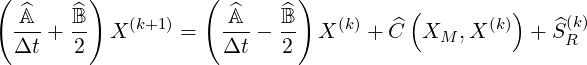
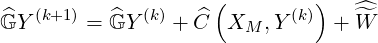
In compact matrix form, the differential equation in the reduced momentum phase space has the following symbolic form

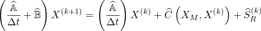(6.2)

where is a single diagonal matrix associated to time differencing, corresponds to the flux divergence and is the first order Legendre correction, and _R is the runaway avalanche source term. Here X^(k) is a vector whose components are the discrete values of the distribution function f₀ at time step , organized as follows

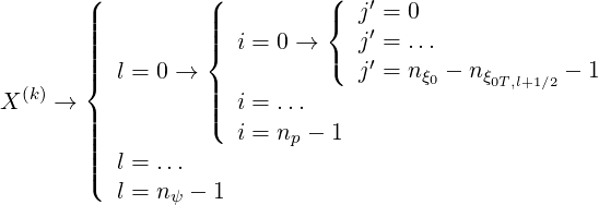(6.3)

while X_M corresponds to the Maxwellian distribution function.

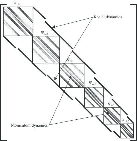
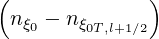Without radial transport, is a block diagonal matrix. Each block, which describes the momentum dynamics at location ψ_l+1∕2, is a square matrice of 15 diagonals whose size n_p×n_p progressively decreases from ψ_1∕2 to ψ_{nξ 0-1∕2} because of the trapped/passing boundary enlarges from the center to the plasma edge, as shown in Fig. 6.1. The main diagonal of is dominant because collisions predominate over other physical processes at each plasma radius.

cmcmcm

Figure 6.1: Qualitative shape of matrix for the Fokker-Planck equation

The introduction of the radial dynamics adds several extra off-diagonals, which connect neighboring blocks corresponding to different radial positions, in addition to the main diagonal which is also modified accordingly. The complexity arises from the fact that trapped electrons may become passing as a result of the radial transport process, and conversely. However, matrix keeps a global banded structure and is still highly sparce, a property that is extensively used for reducing memory storage requirement. Indeed, size of is roughly given by relation

(6.4)

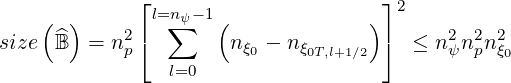
For tokamak with very large aspect ratio, size≈ n_ψ²n_p²n_ξ0² since trapped particle contribution is fairly negligible. In this limit, an upper boundary of the memory size requirement may be estimated. For the reference case, n_ψ = 20, n_p = 200 and n_ξ0 = 200, the total number of coefficients reaches 64 × 10⁺¹⁰, and the needed memory capacity² is 5.12TBytes ! Hopefully, this huge number may be drastically reduced down to 11 × n_ψn_pn_ξ0, since becomes in that limit a simple banded matrix with exactly 11 diagonals. The required memory falls down therefore to 70.4MBytes³, a level which can be easily handled by most computers today.

Crank-Nicholson time scheme

The Crank-Nicholson time scheme is used for time evolution studies of the distribution function f₀. It is second order accurate in time, but this scheme requires usualy Δt∕τ_c^†≈ 1, in order to avoid spurious numerical oscillations towards the steady-state solution f₀. From Eq.6.2, it is straightforward to derive the new matrix form of the Fokker-Planck equation

(6.5)

by just replacing

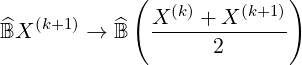(6.6)

since is a linear operator.

6.1.2 Up to first order term: the Drift Kinetic equation

Projected on the numerical distribution function grid, and taking into account of the internal and external boundaries, the 3 - D electron drift kinetic equation may be expressed as

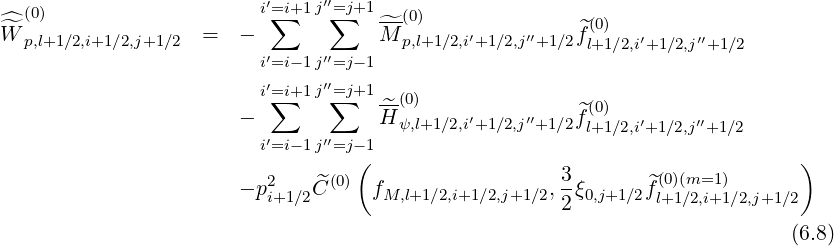
As mentioned in Sec.5.7.2, j →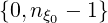, while j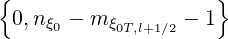^′ → corresponds to the reduced pitch-angle grid which depends of the radial position ψ_l+1∕2, since all the trapped region has been removed. In Eq.6.7, time evolution is not considered, since function g is only determined for steady-state value of . Therefore, iterations to reach the solution only result from the non-linear electron self-collision operator C, that ensures momentum conservation, in order to find a self-consistent solution.

In compact matrix form, the differential equation in the reduced momentum phase space has the following symbolic form

(6.9)

where corresponds to the flux divergence, is the first order Legendre correction and to the contribution of the radial gradient of the distribution function f₀ . Here Y ^(k) is a vector whose components are the discrete values of the distribution function g at iteration step , organized as follows

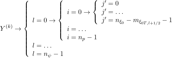(6.10)

and vector X_M is corresponding to the Maxwellian distribution function, as defined in Sec. 6.1.1.

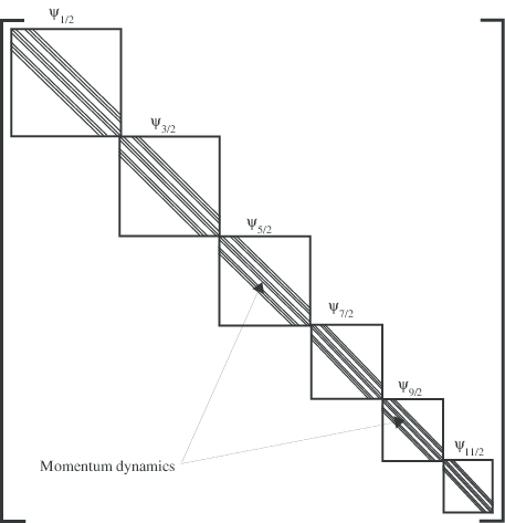
By construction, is simply a block diagonal matrix. Each block, which describes the momentum dynamics at location ψ_l+1∕2, is a square matrice of 9 diagonals whose size n_p×n_p progressively decreases from ψ_1∕2 to ψ_{nξ 0-1∕2} because of the trapped/passing boundary enlarges from the center to the plasma edge, as shown in Fig. 6.2. The main diagonal of is also dominant because collisions predominate over other physical processes at each plasma radius.

cmcmcm

Figure 6.2: Qualitative shape of matrix for the drift kinetic equation

The matrix has a global banded structure with an extremely high sparcity, a property that is also extensively used for memory storage, like for the Fokker-Planck equation (see Sec. 6.1.1). Indeed, the size of is roughlu given by relation

(6.11)

For tokamak with very large aspect ratio, size≈ n_ψ²n_p²n_ξ0² since trapped particle contribution is fairly negligible. In this limit, size≃ size, where is the flux matrix of the Fokker-Planck equation. For the values of n_ψ, n_p and n_ξ0 taken in Sec. 6.1.1, the required memory is approximately 57.6MBytes, a lower level than for the Fokker-Planck equation, since the trapped region is completely removed in the calculations.