 l+1∕2,i+1∕2,j+1∕2(k+1)
 l+1∕2,i+1∕2,j+1∕2(k+1)
 ×
× l+1∕2,i+1∕2,j+1∕2(k+1)
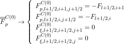
Fokker-Planck equation In this section, only the electron dynamics in momentum space is discussed, at fixed ψl+1∕2. Hence
| l+1∕2,i+1∕2,j+1∕2(k+1) | = l+1∕2,i+1∕2,j+1∕2(k+1) | ||
| -× | |||
| l+1∕2,i+1∕2,j+1∕2(k+1) | (5.43) |
where
 | (5.44) |
Here, diffusion cross-terms between momentum and configuration spaces are neglected, i.e.
Dpψ = Dψp
= Dψp = Dξψ
= Dξψ = Dψξ
= Dψξ = 0. By definition, the discretization procedure must
preserve the conservative nature of the momentum dynamics, as discussed in Sec.
3.5.1, and therefore, careful attention must be paid how to proceed from Eq. 5.4.1, in
particular when diffusion or convection coefficients vary strongly on a grid step. Moreover,
boundary conditions on flux grid must be as much as possible naturaly satisfied by the
discrete form of the Fokker-Planck equation. Indeed, cross-derivatives never satisfy
this condition simultaneously along the momentum and pitch-angle directions, and
consequently additional external boundary conditions must be added to enforce this
condition.
= 0. By definition, the discretization procedure must
preserve the conservative nature of the momentum dynamics, as discussed in Sec.
3.5.1, and therefore, careful attention must be paid how to proceed from Eq. 5.4.1, in
particular when diffusion or convection coefficients vary strongly on a grid step. Moreover,
boundary conditions on flux grid must be as much as possible naturaly satisfied by the
discrete form of the Fokker-Planck equation. Indeed, cross-derivatives never satisfy
this condition simultaneously along the momentum and pitch-angle directions, and
consequently additional external boundary conditions must be added to enforce this
condition.
There are several ways to perform the discretization of the cross-derivatives. Since Dpξ and Dξp
 terms do not contribute to the Maxwellian solution when no external
perturbation is applied, it is not necessary to perform an interpolation between full and
half grids for cross-derivatives in order to ensure a correct numerical flux balance in
momentum space. In that case, the usual procedure is simply to center differences, as
done in this section. However, there is a much more complex approach, but also more
consistent one with respect to the use two grids, one for the fluxes and the other
for the distribution, which is also presented in Appendix F. However, because of its
complexity, it has not been yet implemented in the code even if this approach is in principle
better designed for non-uniform grids with strong localized variations of Dpξ
terms do not contribute to the Maxwellian solution when no external
perturbation is applied, it is not necessary to perform an interpolation between full and
half grids for cross-derivatives in order to ensure a correct numerical flux balance in
momentum space. In that case, the usual procedure is simply to center differences, as
done in this section. However, there is a much more complex approach, but also more
consistent one with respect to the use two grids, one for the fluxes and the other
for the distribution, which is also presented in Appendix F. However, because of its
complexity, it has not been yet implemented in the code even if this approach is in principle
better designed for non-uniform grids with strong localized variations of Dpξ and
Dξp
and
Dξp .
.
The starting point of the discretization procedure is the following expressions
 | =   | ||
+     | |||
+  pDpξ pDpξ  | (5.45) |
 | =   | ||
 | |||
-   | |||
- λDξp λDξp  | (5.46) |
where cross-derivatives terms have been developped directly from analytical formulas, and
considered in separately. Here, it is assumed in an implicit manner that derivatives of pDpξ and
and  λDξp
λDξp exists.
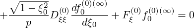
Hence
![(0)|(k+1) m=8
-^q- 2∂f0--|| -^ql+1∕2--∑ [m ]
B0 p ∂t || = B0,l+1∕2 T
l+1∕2,i+1∕2,j+1∕2 m=1](NoticeDKE2765x.png) | (5.47) |
with
![(0)||(k+1)
- p2 D(0) ∂f0-| + p2 F(0) f (0)(k+1)
[1] ---i+1--pp,l+1∕2,i+1,j+1∕2-∂p-|l+1∕2,i+1,j+1∕2----i+1--p,l+1∕2,i+1,j+1∕2-0,l+1∕2,i+1,j+1∕2
T = Δpi+1∕2](NoticeDKE2766x.png) | (5.48) |
![(0)||(k+1)
p2iD (0pp),l+1∕2,i,j+1∕2 ∂f0∂p-|| - p2iFp(0,)l+1∕2,i,j+1∕2f(00),l(+k1+∕21,)i,j+1∕2
T[2] = ---------------------l+1∕2,i,j+1∕2------------------------------
Δpi+1∕2](NoticeDKE2767x.png) | (5.49) |
![( )
∘ -----------∂ pD (0) || (0)||(k+1)
T [3] = + 1- ξ2 -----pξ--|| ∂f0-||
0,j+1∕2 ∂p || ∂ξ |
l+1∕2,i+1∕2,j+1∕2 l+1∕2,i+1∕2,j+1∕2](NoticeDKE2768x.png) | (5.50) |
![|(k+1)
[4] ∘ -----2----- (0) ∂2f0(0)||
T = + 1 - ξ0,j+1∕2pi+1∕2D pξ,l+1∕2,i+1∕2,j+1∕2 ∂p∂ξ ||
l+1∕2,i+1∕2,j+1∕2](NoticeDKE2769x.png) | (5.51) |
T![[5]](NoticeDKE2770x.png) | = -  | ||
+  | (5.52) |
T![[6]](NoticeDKE2774x.png) | =   | ||
+  | (5.53) |
![p (∘ ------ ) || (0)||(k+1)
T[7] = ---i+1∕2----∂-- 1 - ξ20λD (0) | ∂f0--||
λl+1∕2,j+1∕2 ∂ξ0 ξp |l+1∕2,i+1∕2,j+1 ∕2 ∂p |l+1∕2,i+1∕2,j+1∕2](NoticeDKE2778x.png) | (5.54) |
![p ∘ ----------- 2 (0)||(k+1)
T [8] = ---i+1∕2--- 1 - ξ2 λl+1∕2,j+1∕2D (0) ∂--f0-||
λl+1∕2,j+1∕2 0,j+1∕2 ξp,l+1∕2,i+1∕2,j+1∕2∂ ξ0∂p|l+1∕2,i+1∕2,j+1∕2](NoticeDKE2779x.png) | (5.55) |
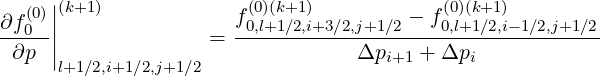
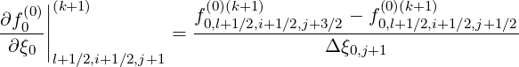
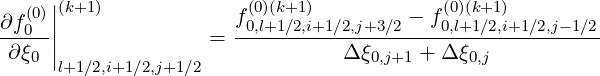
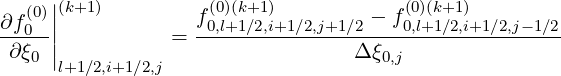
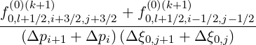
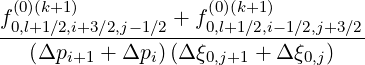
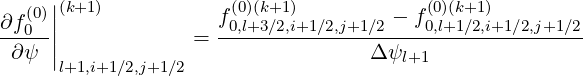
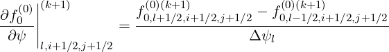
Discrete expressions of the partial derivatives are,
 | (5.56) |
 | (5.57) |
 | (5.58) |
 | (5.59) |
 | (5.60) |
 | (5.61) |
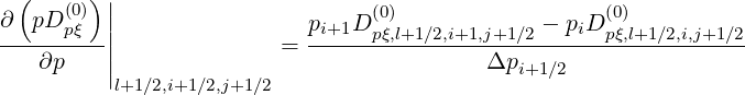
and cross-derivatives
 l+1∕2,i+1∕2,j+1∕2(k+1) l+1∕2,i+1∕2,j+1∕2(k+1) | =  l+1∕2,i+1∕2,j+1∕2(k+1) l+1∕2,i+1∕2,j+1∕2(k+1) | ||
=  | |||
- | (5.62) |
while other derivatives become in discrete form
 | (5.63) |
and
 l+1∕2,i+1∕2,j+1∕2 l+1∕2,i+1∕2,j+1∕2 | |||
=  | |||
- | (5.64) |
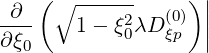
By definition, cross-derivatives are symmetric. Furthermore, the derivative
 | (5.65) |
must be taken on the flux grid in order to fullfil naturally boundary condition at  = 1 and
avoid to specify Dξp
= 1 and
avoid to specify Dξp at this momentum space location. It is a crucial point, especially for
the Lower Hybrid and the Ohmic current drive problems, since this domain of the
momentum space plays a very important role for the determination of the plasma current
level.
at this momentum space location. It is a crucial point, especially for
the Lower Hybrid and the Ohmic current drive problems, since this domain of the
momentum space plays a very important role for the determination of the plasma current
level.
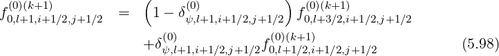
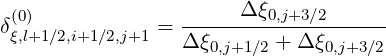
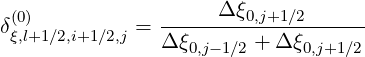
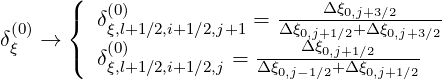
Since the distribution function is defined on the half grid, while fluxes on the full grid, it is
necessary to interpolate, because in some derivatives, values of f0 are taken on the full grid.
In a general way, whatever the detailed value of the weighting factor δ
are taken on the full grid.
In a general way, whatever the detailed value of the weighting factor δ which will be
discussed in the Sec. 5.4.3, one may write for the terms proportional to Dpp
which will be
discussed in the Sec. 5.4.3, one may write for the terms proportional to Dpp and
Fp
and
Fp ,
,
f0,l+1∕2,i+1,j+1∕2 (k+1) (k+1) | =  f0,l+1∕2,i+3∕2,j+1∕2 f0,l+1∕2,i+3∕2,j+1∕2 (k+1) (k+1) | ||
+ δp,l+1∕2,i+1,j+1∕2 f
0,l+1∕2,i+1∕2,j+1∕2 f
0,l+1∕2,i+1∕2,j+1∕2 (k+1) (k+1) | (5.66) |
f0,l+1∕2,i,j+1∕2 (k+1) (k+1) | =  f0,l+1∕2,i+1∕2,j+1∕2 f0,l+1∕2,i+1∕2,j+1∕2 (k+1) (k+1) | ||
+ δp,l+1∕2,i,j+1∕2 f
0,l+1∕2,i-1∕2,j+1∕2 f
0,l+1∕2,i-1∕2,j+1∕2 (k+1) (k+1) | (5.67) |
and for terms proportional to Dξξ and Fξ
f0,i+1∕2,j+1 (k+1) (k+1) | =  f0,l+1∕2,i+1∕2,j+3∕2 f0,l+1∕2,i+1∕2,j+3∕2 (k+1) (k+1) | ||
+ δξ,l+1∕2,i+1∕2,j+1 f
0,l+1∕2,i+1∕2,j+1∕2 f
0,l+1∕2,i+1∕2,j+1∕2 (k+1) (k+1) | (5.68) |
f0,i+1∕2,j (k+1) (k+1) | =  f0,l+1∕2,i+1∕2,j+1∕2 f0,l+1∕2,i+1∕2,j+1∕2 (k+1) (k+1) | (5.69) |
+ δξ,l+1∕2,i+1∕2,j f
0,l+1∕2,i+1∕2,j-1∕2 f
0,l+1∕2,i+1∕2,j-1∕2 (k+1) (k+1) | (5.70) |
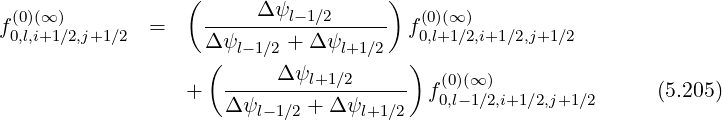
Gathering all terms, corresponding matrix coefficients for the zero order Fokker-Planck equation may be expressed as
 | (5.71) |
where
Mp,l+1∕2,i+3∕2,j+3∕2 | =   Dpξ,l+1∕2,i+1∕2,j+1∕2 Dpξ,l+1∕2,i+1∕2,j+1∕2 | ||
+   Dξp,l+1∕2,i+1∕2,j+1∕2 Dξp,l+1∕2,i+1∕2,j+1∕2 | (5.72) |
Mp,l+1∕2,i+1∕2,j+3∕2 | =   Dpξ,l+1∕2,i+1,j+1∕2 Dpξ,l+1∕2,i+1,j+1∕2 | ||
-  Dpξ,l+1∕2,i,j+1∕2 Dpξ,l+1∕2,i,j+1∕2 | |||
-  Dξξ,l+1∕2,i+1∕2,j+1 Dξξ,l+1∕2,i+1∕2,j+1 | |||
- pi+1∕2  × × | |||
 Fξ,l+1∕2,i+1∕2,j+1 Fξ,l+1∕2,i+1∕2,j+1 | (5.73) |
Mp,l+1∕2,i-1∕2,j+3∕2 | = -  Dpξ,l+1∕2,i+1∕2,j+1∕2 Dpξ,l+1∕2,i+1∕2,j+1∕2 | ||
-  Dξp,l+1∕2,i+1∕2,j+1∕2 Dξp,l+1∕2,i+1∕2,j+1∕2 | (5.74) |
Mp,l+1∕2,i+3∕2,j+1∕2 | = - Dpp,l+1∕2,i+1,j+1∕2 Dpp,l+1∕2,i+1,j+1∕2 | ||
+   × × | |||
 Dξp,l+1∕2,i+1∕2,j+1 Dξp,l+1∕2,i+1∕2,j+1 | |||
-  × × | |||
 Dξp,l+1∕2,i+1∕2,j Dξp,l+1∕2,i+1∕2,j | |||
+   Fp,l+1∕2,i+1,j+1∕2 Fp,l+1∕2,i+1,j+1∕2 | (5.75) |
Mp,l+1∕2,i-1∕2,j+1∕2 | = - Dpp,l+1∕2,i,j+1∕2 Dpp,l+1∕2,i,j+1∕2 | ||
-  × × | |||
 Dξp,l+1∕2,i+1∕2,j+1 Dξp,l+1∕2,i+1∕2,j+1 | |||
+   × × | |||
 Dξp,l+1∕2,i+1∕2,j Dξp,l+1∕2,i+1∕2,j | |||
- δp,i,j+1∕2 δp,i,j+1∕2 F
p,l+1∕2,i,j+1∕2 F
p,l+1∕2,i,j+1∕2 | (5.77) |
Mp,l+1∕2,i+3∕2,j-1∕2 | = -  Dpξ,l+1∕2,i+1∕2,j+1∕2 Dpξ,l+1∕2,i+1∕2,j+1∕2 | ||
-  Dξp,l+1∕2,i+1∕2,j+1∕2 Dξp,l+1∕2,i+1∕2,j+1∕2 | (5.78) |
Mp,l+1∕2,i+1∕2,j-1∕2 | = -  Dpξ,l+1∕2,i+1,j+1∕2 Dpξ,l+1∕2,i+1,j+1∕2 | ||
+   Dpξ,l+1∕2,i,j+1∕2 Dpξ,l+1∕2,i,j+1∕2 | |||
-  Dξξ,l+1∕2,i+1∕2,j Dξξ,l+1∕2,i+1∕2,j | |||
+ pi+1∕2 δξ,l+1∕2,i+1∕2,j δξ,l+1∕2,i+1∕2,j × × | |||
 Fξ,l+1∕2,i+1∕2,j Fξ,l+1∕2,i+1∕2,j | (5.79) |
Mp,l+1∕2,i-1∕2,j-1∕2 | =   Dpξ,l+1∕2,i+1∕2,j+1∕2 Dpξ,l+1∕2,i+1∕2,j+1∕2 | ||
+   Dξp,l+1∕2,i+1∕2,j+1∕2 Dξp,l+1∕2,i+1∕2,j+1∕2 | (5.80) |
For each coefficient, identical diffusion and convection terms appear, which must be evaluated for all physical processes that take place in the plasma (RF, Ohmic electric field, ...),
 | (5.81) |
and
 | (5.82) |
Knock-on source term
The knock-on source term must be evaluated at each radial position ψl+1∕2, and also at each
momentum and pitch-angle positions  in momentum space. However, the
poloidal position of the birth of the secondary electron plays a crucial role in the calculations,
that significantly increases the difficulty of the problem.
in momentum space. However, the
poloidal position of the birth of the secondary electron plays a crucial role in the calculations,
that significantly increases the difficulty of the problem.
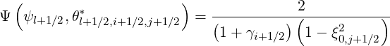
As discussed in Sec. 7.2,
 | (5.83) |
where γ =  , ξ*2 =
  and the poloidal angle θ* is defined by the
relation
and the poloidal angle θ* is defined by the
relation
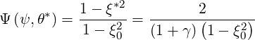 | (5.84) |
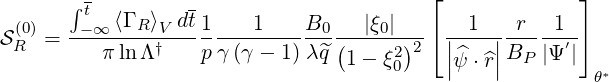
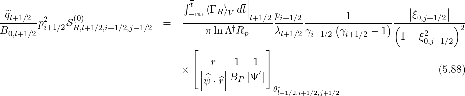
.On the discrete mesh, the source term  R
R at grid point
  becomes
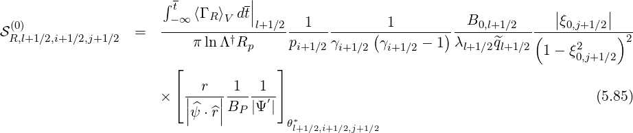
 | (5.86) |
on each flux surface ψl+1∕2. Here
 | (5.87) |
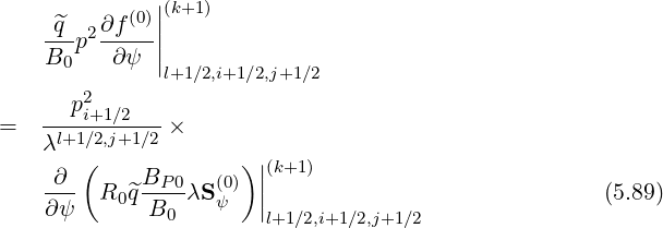
For numerical convenience and for avoiding singularities at boundaries of the integration
domain, the source term R,l+1∕2,i+1∕2,j+1∕2 must be multiplied by a part of the Jacobian J,
i.e.JψJp, and matrix coefficients in the Fokker-Planck equations are
must be multiplied by a part of the Jacobian J,
i.e.JψJp, and matrix coefficients in the Fokker-Planck equations are
In this section, only the electron dynamics in configuration space is discussed, at fixed pi+1∕2 and ξ0,j+1∕2,
 | (5.90) |
since cross-terms between momentum and configuration spaces are neglected, i.e.
Dpψ = Dψp
= Dψp = Dξψ
= Dξψ = Dψξ
= Dψξ = 0.
= 0.
Therefore,
![(0)||(k+1) 2 m=4
q^p2 ∂f--|| = --p-i+1∕2---∑ T[m]
B0 ∂ψ | λl+1∕2,j+1∕2 m=1
l+1∕2,i+1∕2,j+1∕2](NoticeDKE2952x.png) | (5.91) |
with
![[ ]
B2
T[1] = - D (ψ0)ψ,l+1,i+1∕2,j+1∕2 R20,l+1^ql+1-P-0,l+1-λl+1,j+1∕2 ×
B0,l+1
(0)||(k+1)
∂f0--|| ∕Δ ψl+1∕2 (5.92)
∂ψ |l+1,i+1∕2,j+1∕2](NoticeDKE2953x.png)
![[ ]
[2] (0) BP-0,l+1 l+1,j+1∕2
T = F ψ,l+1,i+1∕2,j+1∕2 R0,l+1^ql+1 B0,l+1 λ ×
(0)(k+1)
f0,l+1,i+1∕2,j+1∕2∕Δψl+1∕2 (5.93)](NoticeDKE2954x.png)
![[ B2 ]
T [3] = +D (0) R20,l^ql--P0,lλl,j+1∕2 ×
ψψ,l,i+1∕2,j+1∕2 B0,l
(0)||(k+1)
∂f-0-|
∂ ψ || ∕Δψl+1∕2 (5.94)
l,i+1 ∕2,j+1∕2](NoticeDKE2955x.png)
![[4] (0) [ BP 0,l l,j+1∕2]
T = - F ψ,l,i+1∕2,j+1∕2 R0,lq^l-B--λ ×
0,l
f(00,l)(,ik++11∕)2,j+1∕2∕Δ ψl+1∕2 (5.95)](NoticeDKE2956x.png)
 | (5.96) |
 | (5.97) |
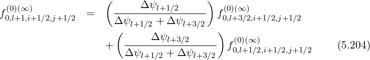
As for the dynamics in momentum space, interpolation between full and half grids must be
performed, since some values of the distribution function f0 must be determined on the flux
grid. Therefore
must be determined on the flux
grid. Therefore

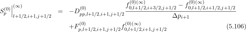
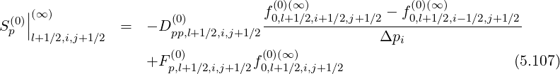
Gathering all terms, matrix coefficients for the zero order Fokker-Planck equation, according to the relation,
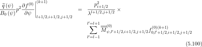
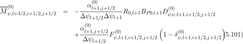
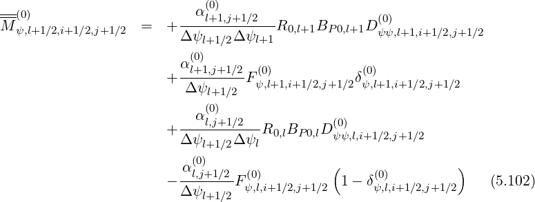
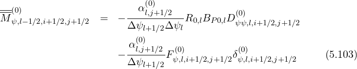
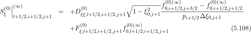
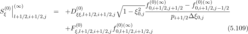
 | (5.104) |
 | (5.105) |
As expected, spatial transport corresponds to a simple tridiagonal matrix.
Momentum grid interpolation
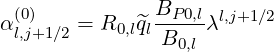
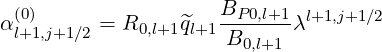
The usual method for determining interpolation coefficients δp,l+1∕2,i+1,j+1∕2 ,
δp,l+1∕2,i,j+1∕2
,
δp,l+1∕2,i,j+1∕2 , δξ,l+1∕2,i+1∕2,j+1
 and δξ,l+1∕2,i+1∕2,j
 so that the distribution function f0
 may be estimated on the full grid (flux grid) from its value on the half grid (distribution grid) is
to satisfy the constraint that numerically, the stationary solution limt→+∞f0
may be estimated on the full grid (flux grid) from its value on the half grid (distribution grid) is
to satisfy the constraint that numerically, the stationary solution limt→+∞f0 = fM is an
exact Maxwellian whithout any external accelerating mechanism (RF wave or Ohmic electric
field). In this case, under the influence of collisional slowing-down and pitch-angle only,
coefficients Dpξ
= fM is an
exact Maxwellian whithout any external accelerating mechanism (RF wave or Ohmic electric
field). In this case, under the influence of collisional slowing-down and pitch-angle only,
coefficients Dpξ = Dξp
= Dξp = 0, and
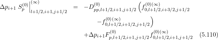
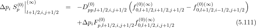
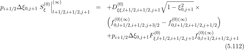
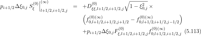
Since this constraint corresponds to the relation
 | (5.114) |
one can deduce,
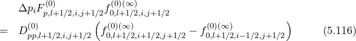
![(0) [( (0) ) (0)(k+1)
Δpi+1Fp,l+1∕2,i+1,j+1∕2 1 - δp,l+1∕2,]i+1,j+1∕2 f0,l+1∕2,i+3∕2,j+1 ∕2
+δ(0) f(0)(k+1)
p,l+1∕2,i+1,j+1∕2(0,l+1∕2,i+1∕2,j+1∕2 )
= D(0) f(0)(∞ ) - f(0)(∞) (5.123)
pp,l+1∕2,i+1,j+1∕2 0,l+1∕2,i+3∕2,j+1∕2 0,l+1∕2,i+1∕2,j+1∕2](NoticeDKE2993x.png)
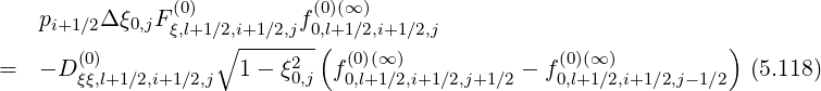
![(0) [( (0) ) (0)(k+1)
ΔpiFp,l+1∕2,i,j+1∕2 1 - δp,l+1∕2,i,j+1∕2 f0,l+1∕2,i+1 ∕2,j+1∕2
(0) (0)(k+1) ]
+ δp,l+1∕2,i,j+1∕2f0,l+1∕2,i- 1∕2,j+1∕2
(0) ( (0)(∞ ) (0)(∞) )
= Dpp,l+1∕2,i,j+1∕2 f0,l+1∕2,i+1∕2,j+1∕2 - f0,l+1∕2,i- 1∕2,j+1∕2 (5.124)](NoticeDKE2994x.png)
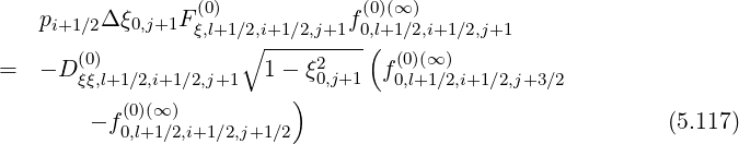
![[( )
pi+1∕2Δξ0,j+1F (ξ0,l)+1∕2,i+1∕2,j+1 1- δ(ξ0,)l+1∕2,i+1∕2,j+1 f0(0,)l+(k1+∕12),i+1∕2,j+3∕2
]
+ δ(ξ0,l)+1∕2,i+1 ∕2,j+1f (00,)l+(k1+∕12),i+1∕2,j+1∕2
∘ ---------(
= - D (0ξξ),l+1∕2,i+1∕2,j+1 1- ξ02,j+1 f(00,l)+(∞1∕)2,i+1∕2,j+3∕2
)
- f0(0,)l+(∞1∕)2,i+1∕2,j+1∕2 (5.125)](NoticeDKE2995x.png)
![[( )
p Δξ F (0) 1- δ(0) f(0)(k+1)
i+1∕2 0,j ξ,l+1 ∕2,i+1∕2,j ξ,l]+1∕2,i+1∕2,j 0,l+1∕2,i+1∕2,j+1∕2
+ δ(0) f (0)(k+1)
ξ,l+1∕2,i+1 ∕2,j0,∘l+1∕2,i+1∕2(,j-1∕2 )
= - D (0) 1- ξ2 f(0)(∞ ) - f(0)(∞) (5.126)
ξξ,l+1∕2,i+1∕2,j 0,j 0,l+1∕2,i+1∕2,j+1∕2 0,l+1∕2,i+1∕2,j-1∕2](NoticeDKE2996x.png)
Hence, the ratios are
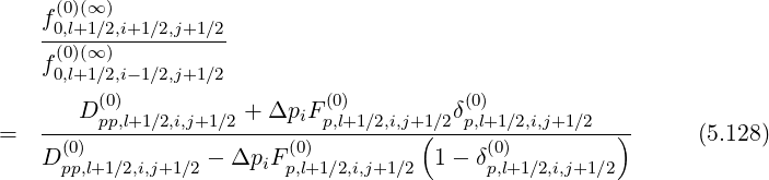
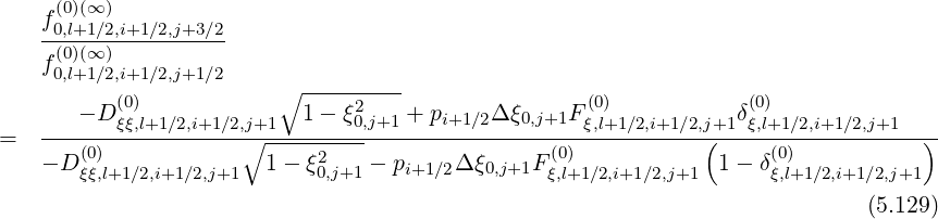
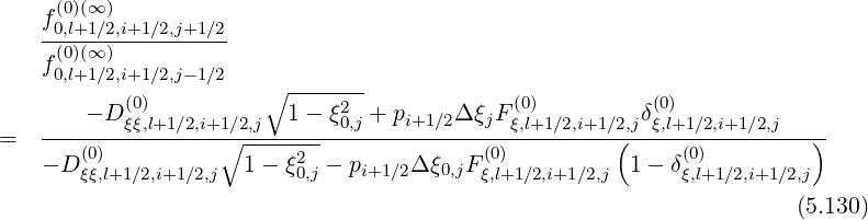
 | (5.131) |
 | (5.132) |
 | (5.133) |
 | (5.134) |
with
 | (5.135) |
 | (5.136) |
 | (5.137) |
 | (5.138) |
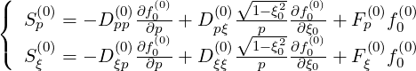
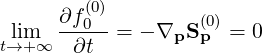
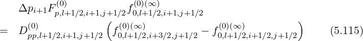
Furthermore, since ∇pSp = 0, one deduces naturally that
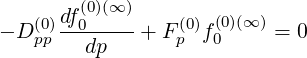 | (5.139) |
 | (5.140) |
and since Fξ = 0 for collisions, because of the isotropic nature of pitch-angle scattering
 | (5.141) |
 | (5.142) |
which indicates that when collisions is the single physical process considered, f0 (∞) is
independent of ξ0. Therefore, ∂∕∂p → d∕dp, and integrating the first equation of (5.141) leads to
the relation
(∞) is
independent of ξ0. Therefore, ∂∕∂p → d∕dp, and integrating the first equation of (5.141) leads to
the relation
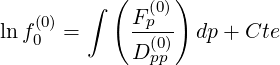 | (5.143) |
Values of f0 (∞) on the respective half grid positions
  and
and
 are then
 | (5.144) |
 | (5.145) |
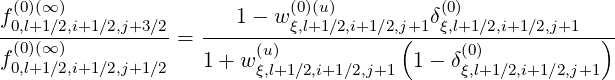
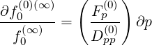
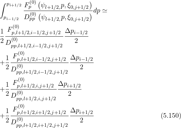
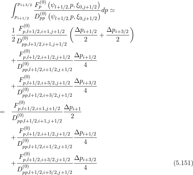
and ratios are finally easily determined
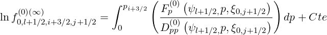
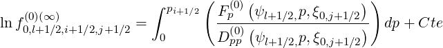
![(0)(∞) [∫ ( ( )) ]
f0,l+1∕2,i+3∕2,j+1∕2- pi+3∕2 F(p0)-ψl+1∕2,p,ξ0,j+1∕2-
(0)(∞) = exp (0)( ) dp
f0,l+1∕2,i+1∕2,j+1∕2 pi+1∕2 Dpp ψl+1∕2,p,ξ0,j+1∕2](NoticeDKE3022x.png) | (5.146) |
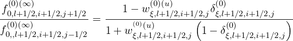
![(0)(∞ ) [ ( ( )) ]
f0,l+1∕2,i+1∕2,j+1∕2 ∫ pi13∕2 F(p0) ψl+1∕2,p,ξ0,j+1∕2
-(0)(∞-)----------= exp -(0)(---------------) dp
f0,l+1∕2,i-1∕2,j+1∕2 pi- 1∕2 Dpp ψl+1∕2,p,ξ0,j+1∕2](NoticeDKE3023x.png) | (5.147) |
while, since f0 (∞) does not depend of ξ0,
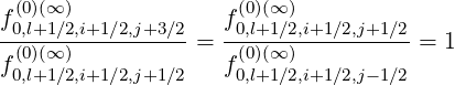 | (5.148) |
It is then straightforward to evaluate coefficients δp,l+1∕2,i+1,j+1∕2 et δp,l+1∕2,i,j+1∕2
 by
the trapezoidal method,
by
the trapezoidal method,
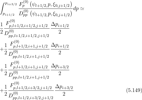
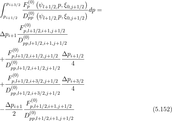
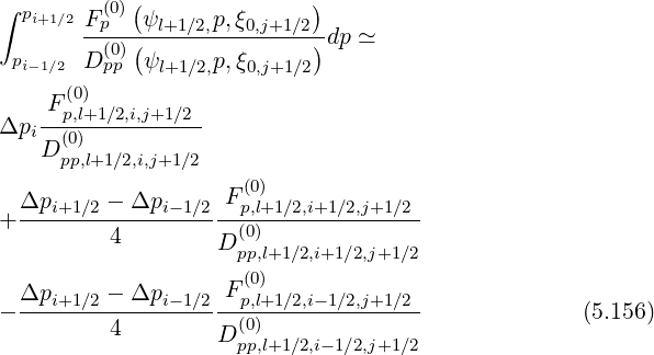
Since
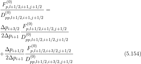
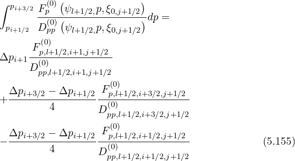
Much as the same way, using index conversion pi+3∕2 → pi+1∕2, pi+1 → pi and pi+1∕2 → pi-1∕2 in the previous relation, one obtains for the second integral,
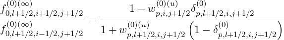
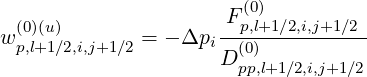
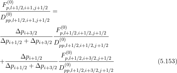
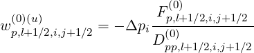
From the two formulations of the ratios
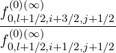 | (5.157) |
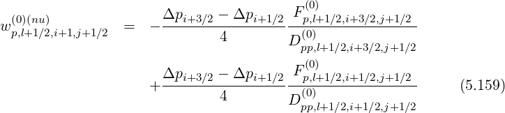
one obtains easily
![(0) -------1-------
δp,l+1∕2,i+1,j+1∕2 = (0)(u)
wp,l+1∕2,i+1,j+1∕2
---------------------1--------------------
- [ (0)(u) (0)(nu) ] (5.158)
exp wp,l+1∕2,i+1,j+1∕2 + w p,l+1∕2,i+1,j+1∕2 - 1](NoticeDKE3037x.png)
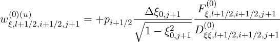
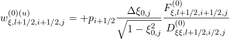
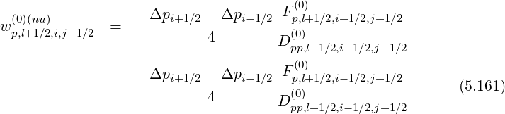
Much in the same way,
![(0) ------1------ ------------------1-------------------
δp,l+1∕2,i,j+1∕2 = (0)(u) - [ (0)(u) (0)(nu) ]
w p,l+1∕2,i,j+1 ∕2 exp wp,l+1∕2,i,j+1∕2 + w p,l+1∕2,i,j+1∕2 - 1](NoticeDKE3039x.png) | (5.160) |
with ß
For a uniform grid, wp,l+1∕2,i,j+1∕2 (nu) = 0, and the well known expression of the Chang
and Cooper function is recovered,
(nu) = 0, and the well known expression of the Chang
and Cooper function is recovered,
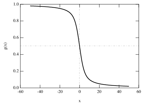
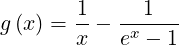 | (5.162) |
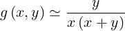
with x = wp (u). In the limit where x ≪ 1, an expansion of the function gives
g
(u). In the limit where x ≪ 1, an expansion of the function gives
g = 0.5 - x∕12 + x3∕720 + O
 with limx→0g
 =
=  , as shwon in Fig.5.2. For a
non-uniform grid, a generalized Chang and Cooper function must be introduced, with two
arguments
, as shwon in Fig.5.2. For a
non-uniform grid, a generalized Chang and Cooper function must be introduced, with two
arguments
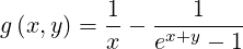 | (5.163) |
where the term y = wp (nu) is zero for the uniform case, as shown in Ref.[?].
With this definition,
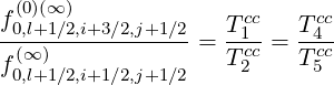 | (5.164) |
where
![⌊
1
Tc1c = 1 - w(p0,l)(+u1)∕2,i+1,j+1∕2⌈ -(0)(u)----------
wp,,l+1∕2,i+1,j+1∕2
⌋
--------------------1---------------------
- [ (0)(u) (0)(nu) ] ⌉ (5.165)
exp wp,l+1∕2,i+1,j+1∕2 + w p,l+1∕2,i+1,j+1∕2 - 1](NoticeDKE3051x.png)
 | (5.166) |
and
![cc -------1------- --------------------1---------------------
T3 = (0)(u) - [ (0)(u) (0)(nu) ]
wp,l+1∕2,i+1,j+1∕2 exp w p,l+1∕2,i+1,j+1∕2 + wp,l+1∕2,i+1,j+1∕2 - 1](NoticeDKE3053x.png) | (5.167) |
whilewith
![w(p0,)(l+u1)∕2,i+1,j+1∕2
Tc4c= ---[--(0)(u)-------------(0)(nu)--------]----
exp w p,l+1∕2,i+1,j+1∕2 + wp,l+1∕2,i+1,j+1∕2 - 1](NoticeDKE3054x.png) | (5.168) |
and
![(0)(u)
Tcc= w(0)(u) + ----[---------wp,l+1∕2,i+1,j+1∕2--------]----
5 p,l+1∕2,i+1,j+1∕2 exp w(0)(u) + w (0)(nu) - 1
p,l+1∕2,i+1,j+1∕2 p,l+1∕2,i+1,j+1∕2](NoticeDKE3055x.png) | (5.169) |
This expression simplifies and becomes
![(0)(∞ )
f0,l+1∕2,i+3∕2,j+1∕2 [ (0)(u) (0)(nu) ]
-(0)(∞-)----------= exp - w p,l+1∕2,i+1,j+1∕2 - w p,l+1∕2,i+1,j+1∕2
f0,l+1∕2,i+1∕2,j+1∕2](NoticeDKE3056x.png) | (5.170) |
Furthermore, when plasma relaxation by collisions is the single process considered, the relation
 | (5.171) |
holds2,
since f0 (∞) must be Maxwellian fM, and one finds
![f(00,l)(+∞1∕)2,i+3 ∕2,j+1∕2 [ Δpi+3 ∕2 - Δpi+1 ∕2 ( )]
-(0)(∞-)----------= exp - Δpi+1pi+1 ---------4-------- pi+3∕2 - pi+1∕2
f0,l+1∕2,i+1 ∕2,j+1∕2](NoticeDKE3061x.png) | (5.172) |
Using identities introduced in Sec. 5.2,
 | (5.173) |
it is easy to demonstrate that
 | (5.174) |
and
 | (5.175) |
Finally, since
![Δpi+3∕2 --Δpi+1-∕2( )
- Δpi+1pi+1 - 4 pi+3∕2 - pi+1∕2
( ) [1 ( ) 1( )]
= - pi+3∕2 - pi+1∕2 -- pi+3∕2 + pi+1∕2 - --Δpi+3 ∕2 - Δpi+1∕2
2 4
Δpi+3∕2 --Δpi+1∕2( )
- 4 pi+3∕2 - pi+1∕2
1-( )( )
= - 2 pi+3∕2 + pi+1∕2 pi+3∕2 - pi+1∕2
1 ( 2 2 )
= - 2- pi+3∕2 - pi+1∕2 (5.176)](NoticeDKE3065x.png)
![f (0)(∞ ) [ p2 - p2 ]
-0,l+1∕2,i+3∕2,j+1∕2= exp - -i+3∕2---i+1∕2-
f (0)(∞ ) 2
0,l+1∕2,i+1∕2,j+1∕2](NoticeDKE3066x.png) | (5.177) |
which is exactly corresponding to a numerical Maxwellian distribution function. Hence, numerical errors do not propagate with the weighting here considered.
Finally, for the non-uniform p grid, the final results for interpolation rules are
 | (5.178) |
with
![(0) 1 1
δp,l+1∕2,i+1,j+1 ∕2 = --(0)(u)--------- - ----[-(0)(u)-------------(0)(nu)--------]----
w p,l+1∕2,i+1,j+1 ∕2 exp wp,l+1∕2,i+1,j+1∕2 + w p,l+1∕2,i+1,j+1∕2 - 1](NoticeDKE3068x.png) | (5.179) |
and
![δ(0) = ------1------ - ----[-------------1--------------]----
p,l+1∕2,i,j+1∕2 w (p0),l(+u1)∕2,i,j+1 ∕2 exp w(p0,)(l+u1)∕2,i,j+1∕2 + w (0p),l(+nu1)∕2,i,j+1∕2 - 1](NoticeDKE3069x.png) | (5.180) |
and where
 | (5.181) |
with
 | (5.182) |
and
 | (5.183) |
Much in the same way,
 | (5.184) |
where
 | (5.185) |
and
 | (5.186) |
It is important to note that since only collisions are considered for evaluating interpolating
coefficients δp , momentum and pitch-angle dynamics are naturally decoupled. Consequently,
the ratios Fp
, momentum and pitch-angle dynamics are naturally decoupled. Consequently,
the ratios Fp ∕Dpp
∕Dpp are only functions of p, and it is the reason why they haves similar values
at different pitch-angle grid points ξ0.
are only functions of p, and it is the reason why they haves similar values
at different pitch-angle grid points ξ0.
By definition, δp must be lower than unity, a condition that is naturaly satisfied for the
uniform momentum grid, as shown in Fig.5.2. However, special care must be taken for the
non-uniform case, since there is no exact cancellation between 1∕x and 1∕
must be lower than unity, a condition that is naturaly satisfied for the
uniform momentum grid, as shown in Fig.5.2. However, special care must be taken for the
non-uniform case, since there is no exact cancellation between 1∕x and 1∕ . In the
limit y < x ≪ 1, it can be easily shown that
. In the
limit y < x ≪ 1, it can be easily shown that
 | (5.187) |
and the condition g ≤ 1 is equivalent to the relation
 | (5.188) |
For a uniform grid, this condition is always fulfilled, since it corresponds to y = 0. For the non-uniform case, it is clear that the range of validity of the extended Chang and Cooper function is much more restricted, since y∕x is finite. Consequently, if x ≃ pΔp is small, y which is proportional to the variation of the grid step as function of p must be significantly smaller which means that the momentum grid is nearly uniform in this region of the phase space. For larger values of x, the condition is easier to satisfy, which indicates that the non-uniformity must be a growing function of the momentum value p, and nearly flat close to p = 0.
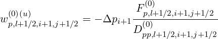
There are however additional limitations on the choice of the momentum for large p values. Indeed, in this domain, other mechanismes are at play, and the usual technique is to extrapolate calculations carried out for collisions to other accelaration mechanismes (Ohmic electric field, RF waves,...), using the generalized weighting factor based on the simple rule,
 | (5.189) |
where ∑ m is the sum over all the physical processes m that take place in the plasma. Since the same syntax may be kept, one obtains simply
 | (5.190) |
and
 | (5.191) |
for the uniform contribution, while for the non-uniform one
 | (5.192) |
and
 | (5.193) |
In that case, the interpolating weights exhibit a dependence with ξ0. This has however a
weak importance for the accuracy of the calculations, since in the domain where fluxes are
strongly modified since usually  effective → 0 in presence of RF quasilinear diffusion. The
Maxwellian distribution function is consequently no more the solution of the Fokker-Planck
equation.
effective → 0 in presence of RF quasilinear diffusion. The
Maxwellian distribution function is consequently no more the solution of the Fokker-Planck
equation.
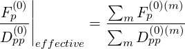
The reason why an effective expression of Fp ∕Dpp
∕Dpp is used for evaluating δp
 where
collisions are not the single process is based on the fact that the Chang and Cooper function
tends towards δp
where
collisions are not the single process is based on the fact that the Chang and Cooper function
tends towards δp ≃
≃ for a uniform mesh when
  effective increases. In that case, it
corresponds exactly to the standard linear interpolation, i.e. the well known arithmetic mean.
The interpolation procedure is therefore consistent with the grid, an important characteristic for
reducing the rate of convergence.
effective increases. In that case, it
corresponds exactly to the standard linear interpolation, i.e. the well known arithmetic mean.
The interpolation procedure is therefore consistent with the grid, an important characteristic for
reducing the rate of convergence.
Unfortunately, such a property is not valid for a non-uniform grid, and the interpolation may be wrong , leading to possible an anomalous behaviour of the code. Consequently, even at larger values of p, only a uniform mesh may provide a consistent solution with the numerical grid in presence of external sources of acceleration. From this analysis, it turns out that the only purpose for using a non-uniform momentum mesh is to establish a link between the fine mesh in the vicinity of p = 0, and a coarse grid in the region where other physical mechanismes are at play. Consequently, the momentum mesh is build from the relation
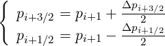
 | (5.194) |
with the recurrence relation
 | (5.195) |
where p0 = 0, Δpnp-1 = pmax∕ and Δp0 is an arbitrary value. Here iref is the index
value corresponding to the transition between the fine and the coarse grids. When Δp0 =
Δpnp-1, the case of an uniform mesh is well recovered, whatever iref. Here Δp0 and iref must be
chosen so that the non-uniform part of the momentum grid is far enough from p = 0 in order the
relation δp
and Δp0 is an arbitrary value. Here iref is the index
value corresponding to the transition between the fine and the coarse grids. When Δp0 =
Δpnp-1, the case of an uniform mesh is well recovered, whatever iref. Here Δp0 and iref must be
chosen so that the non-uniform part of the momentum grid is far enough from p = 0 in order the
relation δp > 1 is satisfied, but also far from the region where external forces play a
role3.
> 1 is satisfied, but also far from the region where external forces play a
role3.
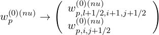
Finally, wp (nu) require evaluations of the quantities at the respective grid points
 and
and  . The usual method to deal with this
problem is shifting indexes, according to the relation
. The usual method to deal with this
problem is shifting indexes, according to the relation
![(l + 1∕2,i+ 1∕2,j + 1∕2) ∈ {[1 : nψ],[1 : np],[1 : nξ]}](NoticeDKE3104x.png) | (5.196) |
and
![{ (l + 1∕2,i- 1∕2,j + 1∕2) ∈ {[1 : nψ],[X, 1 : np - 1],[1 : nξ]}
(l + 1∕2,i+ 3∕2,j + 1∕2) ∈ {[1 : n ],[2 : n ,X ],[1 : n ]}
ψ p ξ](NoticeDKE3105x.png) | (5.197) |
Hence, all quantities have the same size  , which is crucial for the 3 - D matrix
representation. Furthermore, boundary conditions are naturally satisfied with this
technique, since arbitrary values may be attributed to the variable X at these grid
points.
, which is crucial for the 3 - D matrix
representation. Furthermore, boundary conditions are naturally satisfied with this
technique, since arbitrary values may be attributed to the variable X at these grid
points.
Pitch-angle grid interpolation
For the pitch-angle terms, calculation is very simple, and from previous relations, one
deduces directly that wξ,l+1∕2,i+1∕2,j+1 = wξ,l+1∕2,i+1∕2,j
 = 0 since Fξ
 = 0. Therefore,
δξ,l+1:2,i+1∕2,j+1
= 0. Therefore,
δξ,l+1:2,i+1∕2,j+1 may be defined in an arbitrary manner. It is important to note that this
choice is different from the one described in Ref. [?], where the pitch-angle weighting factors are
defined in the same way as for the momentum p. However, it turns out that in presence of RF
waves, this leads sometimes to spurious numerical evolutions, while the simple approach here
described avoid them.
may be defined in an arbitrary manner. It is important to note that this
choice is different from the one described in Ref. [?], where the pitch-angle weighting factors are
defined in the same way as for the momentum p. However, it turns out that in presence of RF
waves, this leads sometimes to spurious numerical evolutions, while the simple approach here
described avoid them.
The most natural way is therefore to perform a linear interpolation, between
f0,l+1∕2,i+1∕2,j+3∕2 (∞) and f0,l+1∕2,i+1∕2,j+3∕2
 (∞), and also between f0,l+1:2,i+1∕2,j+1∕2
 (∞)
and f0,l+1∕2,i+1∕2,j-1∕2
(∞)
and f0,l+1∕2,i+1∕2,j-1∕2 (∞) according to the relations
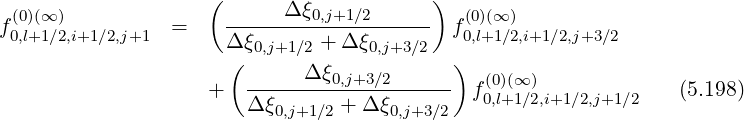
Taking into account of the non-uniform grid steps
 | (5.200) |
 | (5.201) |
and for a uniform grid, the relation δξ,l+1∕2,i+1∕2,j+1 = δξ,l+1∕2,i+1∕2,j
 = 1∕2 are exactly
recovered.
= 1∕2 are exactly
recovered.
Finally, for the non-uniform pitch-angle grid ξ, the interpolation rules are
 | (5.202) |
Furthermore, δξ require evaluations of the quantities at the respective grid points
 and
and  . As for the momentum grid
interpolation, indexes are shifted,
. As for the momentum grid
interpolation, indexes are shifted,
![{ (l + 1∕2,i+ 1∕2,j - 1∕2) ∈ {[1 : nψ],[1 : np],[X,1 : n ξ - 1]}
(l + 1∕2,i+ 1∕2,j + 3∕2) ∈ {[1 : n ],[1 : n ],[2 : n ,X ]}
ψ p ξ](NoticeDKE3125x.png) | (5.203) |
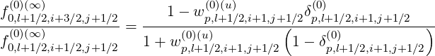
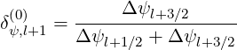
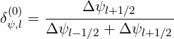
Spatial grid interpolation
The determination of δψ is based on the same method used for δξ
 , since no specific
condition is required for interpolating f0
, since no specific
condition is required for interpolating f0 on the flux grid. A linear interpolation is
considered between f0,l+3∕2,i+1∕2,j+1∕2
on the flux grid. A linear interpolation is
considered between f0,l+3∕2,i+1∕2,j+1∕2 (∞) and f0,l+1∕2,i+1∕2,j+1∕2
 (∞) and also between
f0,l+1∕2,i+1∕2,j+1∕2
(∞) and also between
f0,l+1∕2,i+1∕2,j+1∕2 (∞) and f0,l-1∕2,i+1∕2,j+1∕2
 (∞),
(∞),
 | (5.206) |
 | (5.207) |
For a uniform grid the relation δψ,l+1 = δψ,l
 = 1∕2 is well recovered.
Furthermore, δψ require evaluations of the quantities at the respective grid points
 and
and  . As for the momentum grid
interpolation, indexes are shifted according to the rule
. As for the momentum grid
interpolation, indexes are shifted according to the rule
![{
(l - 1∕2,i+ 1∕2,j + 1∕2) ∈ {[X,1 : nψ - 1],[1 : np ],[1 : nξ]}
(l + 3∕2,i+ 1∕2,j + 1∕2) ∈ {[2 : nψ,X ],[1 : np],[1 : n ξ]}](NoticeDKE3142x.png) | (5.208) |
According to the bounce averaged expression,
 | (5.209) |
and
 | (5.210) |
where each coefficient is the sum of the electron-electron and electron-ion interactions.
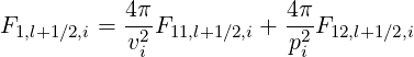
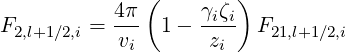
Belaiev-Budker relativistic collision model Here, coefficients corresponding to the Belaiev-Budker collision operator that ranges from non-relativistic to fully relativistic regimes may be expressed as, according to the notation used in Ref.[?],
 | (5.211) |
 | (5.212) |
with
 | (5.213) |
 | (5.214) |
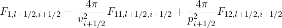
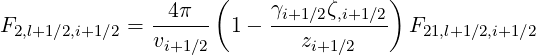
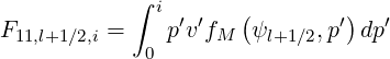
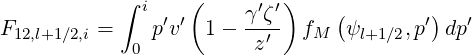
Expressions of coefficients F11,l+1∕2,i+1∕2, F12,l+1∕2,i+1∕2 and F21,l+1∕2,i+1∕2 are
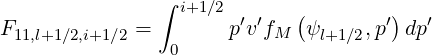 | (5.215) |
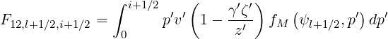 | (5.216) |
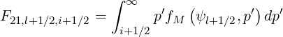 | (5.217) |
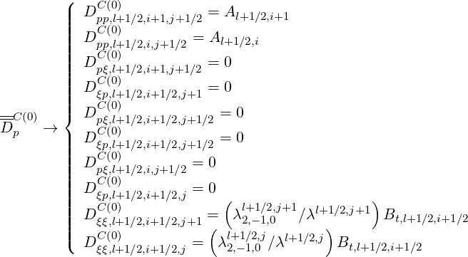
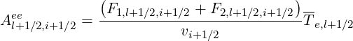
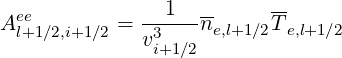
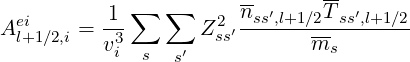
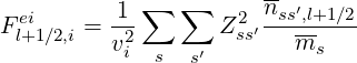
Coefficients Aee and Fee must be also calculated on the flux grids and therefore, according to the previous definition,
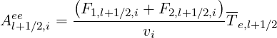 | (5.218) |
and
 | (5.219) |
where
 | (5.220) |
 | (5.221) |
and
 | (5.222) |
 | (5.223) |
 | (5.224) |
for the grid points i, while for the grid points i + 1, one has just to replace i by i + 1 in the set of above expressions.
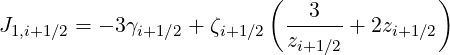
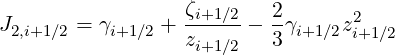
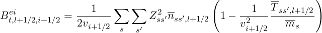
Furthermore, the expression of coefficient Btee is
 | (5.225) |
with
![∑5
Bt1,l+1∕2,i+1∕2 = 4π B [n]
n=1 t1,l+1∕2,i+1∕2](NoticeDKE3160x.png) | (5.226) |
and
![∑5 [n]
Bt2,l+1∕2,i+1∕2 = 4π Bt2,l+1∕2,i+1∕2
n=1](NoticeDKE3161x.png) | (5.227) |
where
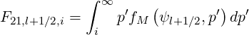
![[1] 1 ∫ i+1∕2 ( )
Bt1,l+1∕2,i+1∕2 = ------- p′2fM ψl+1∕2,p′ dp′
2vi+1∕2 0](NoticeDKE3162x.png) | (5.228) |
![∫ i+1∕2
B [2] = - -----1------ p′4f (ψ ,p′)dp′
t1,l+1∕2,i+1∕2 6vi+1∕2p2i+1∕2 0 M l+1∕2](NoticeDKE3163x.png) | (5.229) |
![[3] 1 ∫ i+1∕2 ′2J′1 ( ′) ′
Bt1,l+1∕2,i+1∕2 = 8γ2---z2---- p γ′fM ψl+1∕2,p dp
i+1∕2i+1∕2 0](NoticeDKE3164x.png) | (5.230) |
![[4] 1 ∫ i+1∕2 ′2J′2 ( ′) ′
Bt1,l+1 ∕2,i+1∕2 = - 4z2---- p γ′fM ψl+1∕2,p dp
i+1∕2 0](NoticeDKE3165x.png) | (5.231) |
![∫ i+1∕2 ′2( ′)
B [5] = ----1--- p-- γ′ - ζ- fM (ψ ,p′)dp′
t1,l+1∕2,i+1∕2 4 γ2i+1∕2 0 γ′ z′ l+1∕2](NoticeDKE3166x.png) | (5.232) |
and
![∫
[1] 1- ∞ p′2- ( ′) ′
B t2,l+1∕2,i+1∕2 = 2 v′ fM ψl+1∕2,p dp
i+1∕2](NoticeDKE3167x.png) | (5.233) |
![[2] γ2i+1∕2 ∫ ∞ p′2 ( )
Bt2,l+1∕2,i+1∕2 = - ------ -′2-′fM ψl+1∕2,p′ dp′
6 i+1∕2 γ v](NoticeDKE3168x.png) | (5.234) |
![∫ ∞ ′2
B[3] = ---J1,i+1∕2--- p---1-fM (ψl+1∕2,p′) dp′
t2,l+1∕2,i+1∕2 8γi+1∕2z2i+1∕2 i+1∕2 v′γ′2](NoticeDKE3169x.png) | (5.235) |
![∫
[4] γi+1∕2J2,i+1∕2- ∞ p-′2-1- ( ′) ′
Bt2,l+1∕2,i+1∕2 = - 4z2 i+1∕2 v′γ ′2fM ψl+1∕2,p dp
i+1∕2](NoticeDKE3170x.png) | (5.236) |
![( ) ∫
[5] ------1----- ζi+1∕2 ∞ ′2 ′ ( ′) ′
B t2,l+1∕2,i+1∕2 = - 4γi+1∕2p2 γi+1∕2 - zi+1∕2 i+1∕2 p v fM ψl+1∕2,p dp
i+1∕2](NoticeDKE3171x.png) | (5.237) |
Here,
 | (5.238) |
 | (5.239) |
with
 | (5.240) |
 | (5.241) |
and
 | (5.242) |
Coefficients A, Bt and F for the Beliaev-Budker relativistic collision operator need to calculate accurately integrals of type
 | (5.243) |
which require a special attention in the vicinity of p = 0, and also of type,
 | (5.244) |
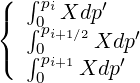
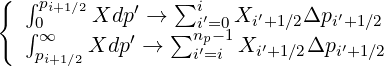
The goal is to ensure an acceptable numerical accuracy which preserves the conservative nature of the equations to be solved by numerical method, without any use of ad-hoc boundary conditions to compensate spurious particle leak arisinf from an improper flux balance at each grid point. For this purpose, a new momentum grid called “super-grid” is introduced, correponding to a refined mesh. Since no specific condition is required as compared to the links between distribution and flux grids, the momentum super-grid is simply defined as a sum of two different meshes for integrals of type ∫ 0pi+1∕2 Xdp′
![[ [
{ s p1∕2- ′ { s }
pi′ ∈ [ nsp ,p1∕2 ,i] → 0{,np - 1 }
psi′ ∈ p1∕2,pi+1∕2 ,i′ → 0,nsp - 1](NoticeDKE3179x.png) | (5.245) |
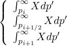
one for very fine calculations below p1∕2, and a second, less refined up to pi+1∕2. For integrals of type ∫ 0piXdp′ and ∫0pi+1Xdp′, the corresponding super-grids are defined in the same way,
![{ [ ]
ps∈ p1∕2,p ,i′ → {0,ns- 1 }
i′s nsp 1′ { s p }
pi′ ∈ [p1,pi],i → 0,np - 1](NoticeDKE3180x.png) | (5.246) |
and
![{ [ ] { }
psi′ ∈ p1n∕s2,p1 ,i′ → 0,nsp - 1
ps∈ [p p,p ],i′ → {0,ns - 1}
i′ 1 i+1 p](NoticeDKE3181x.png) | (5.247) |
It is important to note that p1 correponds to the second point of the grid pi while it is the first one for the grid pi+1, so that numerical integration starts at the same momentum value. Much in the same way, integrals of type ∫ pi∞Xdp′ , ∫ pi+1∕2∞Xdp′ and ∫ pi+1∞Xdp′ are simply defined on the following super-grids
![( ps∈ [p ,p - Δp ],i′ → {0,ns - 1}
|{ i′ [ i max npΔpnp- 1∕2] p { }
| psi′ ∈ pi+1∕2,pmax - -{-2----,i′} → 0,nsp - 1
( ps′ ∈ [pi+1,pmax],i′ → 0,nsp - 1
i](NoticeDKE3182x.png) | (5.248) |
All integrals are performed by the trapezoidal method, even if any more accurate technique like the Simpson method may be used in that case. A crucial point is that integrals exactly end or start at points pi, pi+1∕2 or pi+1 so that no overlap between ∫ 0pi+1∕2 Xdp′ and ∫ pi+1∕2∞Xdp′ can take place. This is especially important to avoid spurious numerical particle leak, that could break the conservative nature of the equations to be solved.
Concerning the first order Legendre correction that ensures momentum conservation, one must calculate
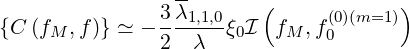 | (5.249) |
on the distribution function grid, where
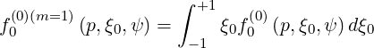 | (5.250) |
as shown in Sec. 4.1.6.
Therefore, by definition,
 | (5.251) |
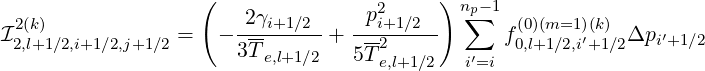
where for the Belaiev-Budker relativistic collision operator,
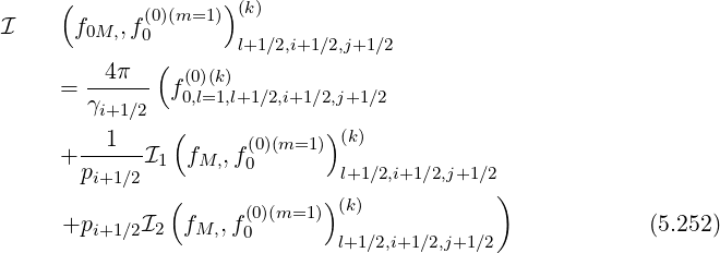

I1 fM,, f0 l+1∕2,i+1∕2,j+1∕2 = I1,l+1∕2,i+1∕2,j+1∕2
n=1](NoticeDKE3187x.png) | (5.253) |
and

2 M, 0 l+1∕2,i+1∕2,j+1∕2 2,l+1∕2,i+1∕2,j+1∕2
n=1](NoticeDKE3188x.png) | (5.254) |
The set of coefficients  1
1![[n]](NoticeDKE3189x.png) is
is
![1 ∑i p3′
I[11],l(+k)1∕2,i+1 ∕2,j+1∕2 = --------- --i+1∕2 f(0,0)l+(1m∕=21,)i′(k+)1∕2Δpi ′+1∕2
3T e,l+1∕2 i′=0γi′+1∕2](NoticeDKE3190x.png) | (5.255) |
 -2γi+1-∕2--∑i 3 (0)(m=1)(k)
I1,l+1∕2,i+1∕2,j+1∕2 = - 3T- pi′+1∕2f0,,l+1∕2,i′+1∕2Δpi ′+1∕2
e,l+1∕2 i′=0](NoticeDKE3191x.png) | (5.256) |
 = -γi+1∕2-- --i′+1∕2 f(0)(m=1)′(k) Δpi ′+1∕2
1,l+1∕2,i+1 ∕2,j+1∕2 5T 2e,l+1∕2 i′=0γi′+1∕2 0,l+1∕2,i+1∕2](NoticeDKE3192x.png) | (5.257) |
 ∑i pi′+1∕2( ζi′+1∕2 ) (0)(m=1 )(k)
I1,l+1∕2,i+1∕2,j+1∕2 = γ′---- γi′+1∕2 - z′---- f 0,l+1∕2,i′+1 ∕2Δpi ′+1∕2
i′=0 i+1∕2 i+1∕2](NoticeDKE3193x.png) | (5.258) |
 γi+1∕2-∑ pi′+1∕2J2,i′+1∕2 (0)(m=1)(k)
I1,l+1∕2,i+1∕2,j+1∕2 = - Te,l+1∕2 γi′+1∕2 z2′ f0,l+1∕2,i′+1∕2Δpi′+1∕2
i′=0 i+1∕2](NoticeDKE3194x.png) | (5.259) |
![γi+1 ∕2p2 - 5T-e,l+1∕2 ∑i p3′
I[16],l(+k)1∕2,i+1 ∕2,j+1∕2 = ------i+1∕22----------- --i+1∕2 f(0,0)l+(1m∕=21,)i′(k+)1∕2Δpi ′+1∕2
6 Te,l+1∕2 i′=0γi′+1∕2
( )
× 1 + --3--- - 3γi′+1∕2ζi′+1∕2 (5.260)
z2i′+1∕2 z3i′+1∕2](NoticeDKE3195x.png)
 γi+1∕2 ∑ i p3i′+1∕2J3,i′+1∕2 (0)(m=1)(k)
I1,l+1 ∕2,i+1∕2,j+1∕2 = --†2-2----- --------------f0,l+1∕2,i′+1∕2Δpi′+1∕2
2βthTe,l+1∕2i′=0 γi′+1∕2 zi′+1∕2](NoticeDKE3196x.png) | (5.261) |
 --γi+1∕2--∑i p3i′+1∕2J1,i′+1-∕2- (0)(m=1 )(k)
I1,l+1∕2,i+1∕2,j+1∕2 = 2T- γ′ z2′ f0,l+1∕2,i′+1 ∕2Δpi ′+1∕2
e,l+1∕2 i′=0 i+1∕2 i+1∕2](NoticeDKE3197x.png) | (5.262) |
 = --i+1∕2- pi′+1∕2 γi′+1∕2ζi′+1∕2 - 1 f(0)(m=1)′(k) Δpi′+1 ∕2
1,l+1∕2,i+1∕2,j+1∕2 Te,l+1∕2 i′=0γi′+1∕2 zi′+1 ∕2 0,l+1∕2,i+1∕2](NoticeDKE3198x.png) | (5.263) |
 γ2i+1∕2 ∑i p3i′+1∕2 J4,i′+1∕2 (0)(m=1 )(k)
I1,l+1∕2,i+1∕2,j+1∕2 = -----†2--2---- ------ -------f0,l+1∕2,i′+1∕2Δpi′+1∕2
12βthT e,l+1∕2 i′=0γi′+1∕2 zi′+1∕2](NoticeDKE3199x.png) | (5.264) |
and the coefficients 2![[n]](NoticeDKE3200x.png) are
are
 1 np∑-1 1 (0)(m=1)(k)
I2,l+1∕2,i+1∕2,j+1∕2 = --------- γ′----f0,l+1∕2,i′+1∕2Δpi′+1∕2
3Te,l+1∕2 i′=i i+1∕2](NoticeDKE3201x.png) | (5.265) |
 | (5.266) |
∕2,i+1∕2,j+1∕2 = γi+1 ∕2 - -i+1∕2- -21--- ---1--f0(0,)l+(m1=∕12,i)(′+k1)∕2Δpi′+1∕2
zi+1∕2 pi+1∕2 i′=i γi′+1∕2](NoticeDKE3203x.png) | (5.267) |
 J2,i+1∕2 n∑p- 1 (0)(m=1)(k)
I2,l+1∕2,i+1∕2,j+1∕2 = - -2----------- f0,l+1∕2,i′+1∕2Δpi′+1∕2
zi+1∕2Te,l+1∕2 i′=i](NoticeDKE3204x.png) | (5.268) |
 = 1+ --3---- 3γi+1∕2ζi+1∕2 ----1----
2,l+1 ∕2,i+1∕2,j+1∕2 z2i+1∕2 z3i+1∕2 6T-2
( -- e),l+1 ∕2
np∑-1 γi′+1 ∕2p2i′+1∕2 - 5Te,l+1∕2 (0)(m=1)(k)
× ---------γ′------------ f0,l+1∕2,i′+1∕2Δpi′+1∕2
i′=i i+1∕2
(5.269)](NoticeDKE3205x.png)
 J3,i+1∕2 J1,i+1∕2
I2,l+1∕2,i+1∕2,j+1∕2 = --------†2-2-----+ --2-----------
2zi+1∕2βthTe,l+1∕2 2zi+1∕2T e,l+1∕2
) np∑-1
- -----J4,i+1∕2------ × f(0)(m=1)′(k) Δp ′
12zi+1∕2β†t2hT2e,l+1∕2 i′=i 0,l+1∕2,i+1∕2 i+1∕2
(5.270)](NoticeDKE3206x.png)
 1 (γi+1∕2ζi+1∕2 )
I2,l+1∕2,i+1∕2,j+1∕2 = -2----------- ---z------- - 1
pi+1∕2Te,l+1∕2 i+1 ∕2
np∑-1 p2′
× -i+1∕2f(00,l)(+m1=∕12,)i′(+k)1∕2Δpi′+1∕2 (5.271)
i′=i γi′+1∕2](NoticeDKE3207x.png)
 | (5.272) |
 | (5.273) |
and
 | (5.274) |
For this case, integrals are simply calculated according to the rule
 | (5.275) |
so that f0,l+1∕2,i+1∕2,j+1∕2

 must not be interpolated between 0 and pi+1∕2 for refined
calculations as done for coefficients Aee, Btee and Fee. Even if by this techniqe, the numerical
accuracy is poor in the vicinity of p = 0, consequences are fairly negligible for the momentum
conservation and the current level, since first-order Legendre corrections are weighted by
p.
must not be interpolated between 0 and pi+1∕2 for refined
calculations as done for coefficients Aee, Btee and Fee. Even if by this techniqe, the numerical
accuracy is poor in the vicinity of p = 0, consequences are fairly negligible for the momentum
conservation and the current level, since first-order Legendre corrections are weighted by
p.
Relativistic Maxwellian background The relativistic Maxwellian background corresponds to that case where the first order Legendre correction for momentum conservation is neglected. Matrix coeffients Aee, Btee and Fee determined in the previous section are used.
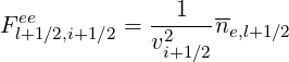
Non-relativistic Maxwellian background For this case, matrix coefficients are
![ee ne,l+1∕2 [ ( ) ′( )]
A l+1∕2,i+1∕2 = 2v----u2--------- erf ul+1∕2,i+1 ∕2 - ul+1 ∕2,i+1∕2erf ul+1∕2,i+1∕2
i+1∕2 l+1∕2,i+1∕2](NoticeDKE3215x.png) | (5.276) |
![n- [ ( ) ( )]
Flee+1∕2,i+1∕2 = --e,2l+1∕2 erf ul+1∕2,i+1∕2 - ul+1∕2,i+1∕2erf′ ul+1∕2,i+1∕2
vi+1∕2](NoticeDKE3216x.png) | (5.277) |
and
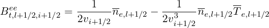
Bt,l+1∕2,i+1∕2ee =   | |||
![( )]
+ul+1∕2,i+1∕2erf′ ul+1∕2,i+1∕2](NoticeDKE3219x.png) | (5.278) |
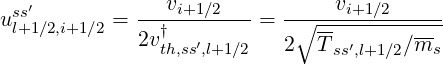
where
 | (5.279) |
For values of the matrix coefficients Aee, Btee and Fee on the momentum flux grids, one just has to replace i + 1∕2 by i or i + 1.
High velocity limit Though the high velocity limit corresponds to a restricted range of application regarding the full collision operator, it can contribute to useful comparisons with some theoretical calculations. Therefore, this possibility has been implemented in the code. In that case, expressions of the coefficients are greatly simplified,
 | (5.280) |
and
 | (5.281) |
while
 | (5.282) |
Since no integrals appear in the coefficients, the expressions at momentum flux grid points i and i + 1 can be obtained in a straightforward manner, by just replacing i + 1∕2 by the corresponding index values. In that limit, the first-order Legendre correction is neglected. In the calculations, both electron-electron and electron-ion collision model in the high velocity limit are used for a consistent description of the collisions.
Non-relativistic Lorentz model This very simple case corresponds to
 | (5.283) |
and also on the momentum flux grid points i and i + 1. Obviously, the first-order Legendre correction is also neglected in that case.
Non-relativistic Maxwellian background In that case matrix coefficients are
![ei ---1---∑ ∑ -----1-----[ ( ss′ )
A l+1∕2,i+1∕2 = 2vi+1∕2 uss′2 erf ul+1∕2,i+1∕2
s s′ l+(1∕2,i+1∕2 )]
- ul+1∕2,i+1∕2erf′ uss′ Z2 ′nss′,l+1∕2 (5.284)
l+1∕2,i+1∕2 ss](NoticeDKE3225x.png)
Fl+1∕2,i+1∕2ei =  ∑
s ∑
s′ ∑
s ∑
s′ | |||
![ss′ ′( ss′ )]
- ul+1∕2,i+1∕2erf ul+1∕2,i+1∕2](NoticeDKE3228x.png) Zss′2 Zss′2 | (5.285) |
and
![ei ---1---∑ ∑ -----1-----[( ss′2 ) ( ss′ )
Bt,l+1∕2,i+1∕2 = 4vi+1∕2 uss′2 2ul+1∕2,i+1∕2 - 1 erf ul+1∕2,i+1∕2
s s′ l+(1∕2,i+1∕2 ) ]
+uss′ erf′ uss′ Z2 ′nss′,l+1∕2 (5.286)
l+1∕2,i+1∕2 l+1∕2,i+1∕2 ss](NoticeDKE3230x.png)
In the case Tss′,l+1∕2 = 0, to avoid a singularity,
 | (5.287) |
while
 | (5.288) |
since erf = 1 and erf′
 = 0.
= 0.
Finally, for values of the matrix coefficients Aei,Fei and Btei on the momentum flux grids, one just has to replace i + 1∕2 by i or i + 1.
High-velocity limit In this limit, matrix coefficients are
 | (5.289) |
 | (5.290) |
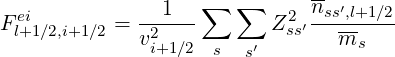
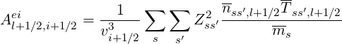
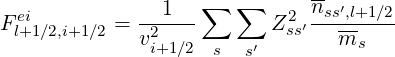
The double sum ∑ s ∑ s′ takes into account of all ions species s in ionization state s′. Here, nss′,l+1∕2 is the normalized ion density at ψl+1∕2, as introduced in Sec. 6.3.1, and ms is the ion rest mass normalized to the electron rest mass me.
Coefficients Aei and Fei must be also calculated on the flux grids and therefore, according to the previous definition,
 | (5.291) |
and
 | (5.292) |
for the grid points i, while for the grid points i + 1, one has just to replace i by i + 1 in the set of above expressions.
Furthermore, the expression of coefficient Btei is
 | (5.293) |
Non-relativistic Lorentz model In that limit
 | (5.294) |
while
 | (5.295) |
A straightforward extrapolation may be done for the momentum flux grid i by i + 1.
According to the bounce averaged expression,
 | (5.296) |
and
 | (5.297) |
where E∥0,l+1∕2 is the parallel component of the Ohmic electric field along the magnetic field line direction normalized to the Dreicer field taken at the poloidal position where the magnetic field B is minimum, as explained in Sec.4.2.
It is important to recall that the Ohmic electric field operator has a cylindrical symmetry,
while the description of the electron dynamics in momentum space is based on the
spherical symmetry of the collision operator. As a consequence, there is a fundamental
contradiction for the internal boundary at p = 0 where p2Sp = 0. Indeed, for large
values of E∥0, the maximum of the distribution function f0 is no more at p = 0,
but may be significantly shifted along the axis p⊥ = 0. Since in that extrem case
p2Sp≠0 at p = 0 while it is naturally enforced to be null by construction with the
grid definition, the distribution function has a wrong shape close to p = 0 and the
conservative scheme is no more preserved. It is also important to note that the external
boundary ∂f0
is no more at p = 0,
but may be significantly shifted along the axis p⊥ = 0. Since in that extrem case
p2Sp≠0 at p = 0 while it is naturally enforced to be null by construction with the
grid definition, the distribution function has a wrong shape close to p = 0 and the
conservative scheme is no more preserved. It is also important to note that the external
boundary ∂f0 ∕∂ξ0 = 0 at ξ0 = 0 is also no more consistent with initial bounce
averaged assumptions, which represents also an important failure of the use of the
code.
∕∂ξ0 = 0 at ξ0 = 0 is also no more consistent with initial bounce
averaged assumptions, which represents also an important failure of the use of the
code.
Consequently, in order to avoid a misuse of the code, the range of validity of E∥0 is restricted so that condition
 | (5.298) |
is fullfiled at p∕pth = 1. Using the high-velicity limit of the collision operator, this corresponds roughly to
 | (5.299) |
since ne ≃ 1 in normalized units, as defined in Sec.6.3.1. Consequently, flux surface averaged
value of the Ohmic electric field  should be restricted to 0.05, in Dreicer units. A warning is
indicated when this value is exceeded.
should be restricted to 0.05, in Dreicer units. A warning is
indicated when this value is exceeded.
From the expressions given in Sec. 4.3.7, the components of the tensor DpRF are
are
![DRF (0) = ∑+ ∞ ∑ (1 - ξ2 )DRF (0)
pp,l+1∕2,i+1,j+1∕2 ∑ n=-∞∑ b 0,j+1∕2RFb(,n0,)l+1∕2,i+1,j+1∕2
DRFpp,(0l+)1∕2,i,j+1∕2 = +n∞=-∞ b(1 - ξ20,j+1∕2)D b,n,l+1∕2,i,j+1∕2
∑ ∑ ∘1-ξ20,j+1∕2 [ nΩ ]--RF(0)
DRFpξ,(0l+)1∕2,i+1,j+1∕2 = +n∞=-∞ b- -ξ0,j+1∕2--- 1- ξ20,j+1∕2 - --0,l+1ω∕b2,i+1- D b,n,l+1∕2,i+1,j+1∕2
∑ ∑ ∘1-ξ2---[ ]--
DRFξp,(0l+)1∕2,i+1∕2,j+1 = +n∞=-∞ b- -ξ--0,j+1-1 - ξ20 - nΩ0,l+1ω∕2,i+1∕2 DRFb,n(,l0+)1∕2,i+1∕2,j+1
∘01,j+-1ξ2----[ b ]--
DRF (0) = ∑+n=∞-∞ ∑b - -----0,j+1∕2 1 - ξ20 - nΩ0,l+1∕2,i+1∕2 DRFb,n(,0l+)1∕2,i+1∕2,j+1∕2
pξ,l+1∕2,i+1∕2,j+1∕2 ∘ ξ0,j+12∕2--[ ωb ]
DRF (0) = ∑+ ∞ ∑ - --1-ξ0,j+1∕2 1 - ξ2- nΩ0,l+1∕2,i+1∕2 DRF (0)
ξp,l+1∕2,i+1∕2,j+1∕2 n= -∞ ∘b---2ξ0,j+1∕[2 0 ω]b b,n,l+1∕2,i+1∕2,j+1∕2
DRF (0) = ∑+ ∞ ∑ ---1-ξ0,j+1∕2 1 - ξ2- nΩ0,l+1∕2,i DRF (0)
pξ,l+1∕2,i,j+1∕2 n=-∞ b ∘ ξ0,j+1∕2 0 ωb b,n,l+1∕2,i,j+1∕2
RF(0) ∑+ ∞ ∑ --1-ξ20,j[ 2 nΩ0,l+1∕2,i+1∕2]--RF(0)
D ξp,l+1∕2,i+1∕2,j = n=-∞ b - ξ0,j [ 1 - ξ0,j - ωb ] D b,n,l+1∕2,i+1∕2,j
DRF (0) = ∑+ ∞ ∑ -21-- 1- ξ2 - nΩ0,l+1∕2,i+1∕2 2DRF (0)
ξξ,l+1∕2,i+1∕2,j+1 n=-∞ b ξ0,[j+1 0,j ωb ]2-- b,n,l+1∕2,i+1∕2,j+1
DRF (0) = ∑+ ∞ ∑ -12- 1- ξ2 - nΩ0,l+1∕2,i+1∕2 DRF (0)
ξξ,l+1∕2,i+1∕2,j n=-∞ b ξ0,j 0,j ωb b,n,l+1∕2,i+1 ∕2,j](NoticeDKE3251x.png) | (5.300) |
and
 | (5.301) |
where Ω0,l+1∕2,i+1∕2 is the electron cyclotron frequency taken at the minimum B value
 | (5.302) |
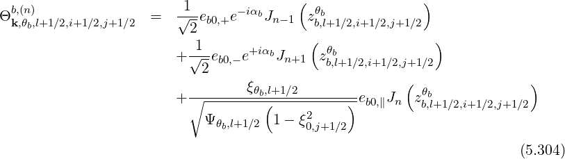
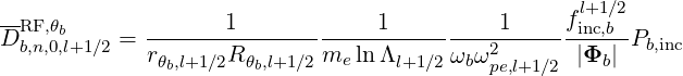
Here the dependence of Ω0,l+1∕2,i+1∕2 with the index i arises from relativistic down-shift. The indexes n and b correspond respectively to the wave harmonics and the narrow beam label (for ray-tracing calculations). The discrete expression of the quasilinear diffusion coefficient Db,n,l+1∕2,i+1∕2,j+1∕2RF(0) is
![-- r B θb ξ2
DRFb,n(0,l)+1∕2,i+1∕2,j+1∕2 = --γi+1|∕2pTe--|-------1---------θb,l+1∕2--l+1∕2-----0,j+12----
pi+1∕2|ξ0,j+1∕2|λl+1∕2,j+1∕2^ql+1∕2 Rp B θPb,l+1∕2ξ2θb,l+1∕2,j+1∕2
--RF,θb
× Ψ θb,l+1∕2D b,n,0,l+12H (θb - θmin)H (θmax - θb)
[ ∑ ] ( )| |2
× 1- δ Nb∥ - N∥θbres,l+1∕2,i+1∕2,j+1∕2 ||Θbk,,(nθ),l+1∕2,i+1∕2,j+1∕2||
2 σ T b
(5.303)](NoticeDKE3254x.png)
 | (5.305) |
 | (5.306) |
with
 | (5.307) |
and
 θb,l+1∕2 θb,l+1∕2 | =  (ψl+1∕2,θb) (ψl+1∕2,θb) | (5.308) |
| rθb,l+1∕2 | = r | (5.309) |
| Rθb,l+1∕2 | = R | (5.310) |
| Bl+1∕2θb | = B | (5.311) |
| BP,l+1∕2θb | = BP  | (5.312) |
| Ψθb,l+1∕2 | =  = =  | (5.313) |
| ξθb,l+1∕2,j+1∕2 | = ξ = σ = σ | (5.314) |
All coefficients corresponding to different indexes may be obtained readily by performing the
adequate index transformation, i + 1∕2 → and j + 1∕2 →