on which the drift
kinetic equation is solved is characterized by three dimensions
on which the drift
kinetic equation is solved is characterized by three dimensions  , and, the time evolution
is introduced with the parameter t.
, and, the time evolution
is introduced with the parameter t.
The drift kinetic equation may be solved by different numerical techniques. Here one of the most
natural approach is described, namely the finite difference method, which is based on the
transformation of a differential equation into an algebraic one. The volume on which the drift
kinetic equation is solved is characterized by three dimensions , and, the time evolution
is introduced with the parameter t.
Since the drift kinetic equation is expressed in conservative form, it is natural to define the grids for the flux S grid as the starting point of the numerical calculations.
![(| t ∈ [0,+ ∞ ],k → {0,nt}
|{ ψk ∈ [0,ψ ],l → {0,n }
S(tk,ψl,pi,ξ0,j) → l a ψ
||( pi ∈ [0,pmax],i → {0,np}
ξ0,j ∈ [- 1,1],j → {0,nξ0}](NoticeDKE2685x.png) | (5.21) |
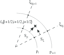
This grid system defines a set of cells of non-uniform sizes characterized by index numbers which, by definition, are integers. The distribution function f is represented by its values inside these cells, as shown in Fig.5.1 for the momentum dynamics. With this form, the conservative nature of the problem is preserved numerically, avoiding the occurence of spurious numerical fluxes which lead to wrong estimate of the solution.
![(
| tk ∈ [0,+ ∞ ],k → {0,nt}
|||| [ Δ-ψ1∕2 Δψnr-1∕2]
( ) |{ ψl+1∕2 ∈ [0 + 2 ,a - 2 ] ,l → {0,nψ - 1}
f tk,ψl+1∕2,pi+1∕2,ξ0j+1∕2 → pi+1∕2 ∈ Δp1∕2,pmax - Δpnp-1∕2- ,i → {0,np - 1}
|||| [ 2 2Δξ ]
||( ξ0j+1∕2 ∈ - 1+ Δξ0,1∕2,1 - --0,nξ0-1∕2 ,j → {0,nξ0 - 1}
2 2](NoticeDKE2686x.png) | (5.22) |
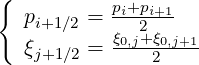
Momentum dynamic in p and pitch-angle ξ0 being independent, the position of pi+1∕2 in between pi and pi+1, and of ξ0,j+1∕2 in between ξ0,j and ξ0,j+1 is an arbitrary choice. The most simple and natural one is to place the point where the distribution function f is determined exactly in the middle of the cell,
 | (5.23) |
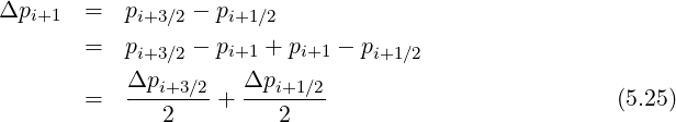
Then, intervals on the different grids are
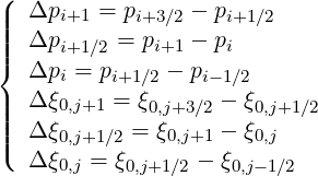 | (5.24) |
where
It is important to note that the need of a non-uniform momentum grid is justified by the 3 - D approach of the numerical code. Indeed, since all radii are considered at each time step, ans since plasma temperature is usually much lower at the edage than at the plasma center, this requires a finer mesh close to p = 0, in order to describe momentum dynamics at all radii with a single p grid. Moreover, this argument holds for the case of multi-species drift kinetic calculations, since ion velocities are much lower than electron ones.
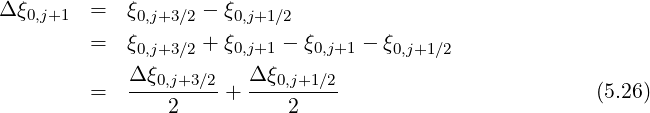
By an appropriate bounce averaging, the number of dimension is reduced to one, i.e. the radial one. As for the dynamics in momentum space, the point where the distribution function f is determined is chosen exactly in the middle of the cell,
 | (5.27) |
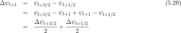
and the intervals on the different grids are,
 | (5.28) |
where
When the bounce averaged drift kinetic equation is solved, the distribution function
f ≡ f
≡ f is determined by definition at the poloidal angle value where the magnetic
field is minimal on a given magnetic flux surface as shown in Sec.2.2.1. It is indeed the only
common poloidal point on the magnetic flux surface that is crossed by trajectories of both
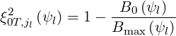
trapped and circulating electrons. In momentum space, the dynamics of trapped and
passing particles is characterized by an interval boundary which is defined by the
relation
is determined by definition at the poloidal angle value where the magnetic
field is minimal on a given magnetic flux surface as shown in Sec.2.2.1. It is indeed the only
common poloidal point on the magnetic flux surface that is crossed by trajectories of both
trapped and circulating electrons. In momentum space, the dynamics of trapped and
passing particles is characterized by an interval boundary which is defined by the
relation
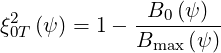 | (5.30) |
From relation (5.30), it is clear that momentum and radial grids are no more fully independent. In order to achieve calculations with a high numerical accuracy, the pitch-angle flux grid is therefore chosen so that there exists an index number jl where the following condition is exactly fullfiled1,
 | (5.31) |
With this definition, the trapped passing boundaries are consistent with both pitch-angle and
spatial flux grids. Obviously, the use of a non-uniform pitch-angle flux grid is fully necessary,
because of this numerical requirement. Hence, if the number of radial points for the flux grid is
arbitrary by definition, the number of points for the pitch-angle grid has a lower limit. It is
straightforward to give a rough estimate, in order to evaluate the numerical size of the objects in
the code. Let nψ being the number of flux grid points, nξ0 ≥ 6nψ + 7, since at least each trapped
passing boundary on the pitch-angle flux grid must be framed by two consecutive neighbors
points, on each side, for ξ0 > 0 et ξ0 ≤ 0 domains. In addition, accurate calculations
must be performed at ξ0 (3 points) et at  = 1 (4 points). Hence, for nψ = 30,
nξ0 ≥ 187.
= 1 (4 points). Hence, for nψ = 30,
nξ0 ≥ 187.
Time evolution is also projected on a numerical grid,
 | (5.32) |
which is taken uniform for two reasons. First, in the numerical approach here considered, the
algorithm, as discussed in Sec. 6.1.1, is mainly dedicated to the fast determination
of the asymptotic stationary solution limt→+∞f = f
= f
 , and
therefore time step values must fulfill the condition Δt ≫ 1. In this limit, the time t
used in the iterative procedure because of the weak non-linearities of the collision
operator, acts mainly as a regularization parameter, when matrix to be inverted is close
to be ill-conditionned. Furthermore, with a non-uniform time grid, matrix must be
calculated at each time step, which prevents the use of the very efficient incomplete LU
matrix factorization technique, as discussed in Sec. 6.2.2, a procedure that allows to
reduce considerably computer time consumption. Since the code is expected to be
incorporate in a chain of codes, in order to obtain self-consistent magnetic equilibrium, wave
propagation and kinetic calculations, this is therefore the only choice that can be
considered.
, and
therefore time step values must fulfill the condition Δt ≫ 1. In this limit, the time t
used in the iterative procedure because of the weak non-linearities of the collision
operator, acts mainly as a regularization parameter, when matrix to be inverted is close
to be ill-conditionned. Furthermore, with a non-uniform time grid, matrix must be
calculated at each time step, which prevents the use of the very efficient incomplete LU
matrix factorization technique, as discussed in Sec. 6.2.2, a procedure that allows to
reduce considerably computer time consumption. Since the code is expected to be
incorporate in a chain of codes, in order to obtain self-consistent magnetic equilibrium, wave
propagation and kinetic calculations, this is therefore the only choice that can be
considered.