In order to use parameters without dimensions in the calculations, all of them are normalized to reference values. Here temperature and densities correspond to flux surface-averaged values, though the usual bracket notation is not introduce, for sake on simplicity.
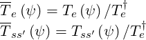
Normalized temperatures, are defined by the relations
|
| (6.36) |
where the subscripts e stands for electrons and ss′ for ion species s in the ionization state s′,
whose charge is Zss′qe. Here, both Te and Te† have defined units, while Te† is the reference
value for the normalization. According to this rule, the normalized densities are defined in the
same way
and Te† have defined units, while Te† is the reference
value for the normalization. According to this rule, the normalized densities are defined in the
same way
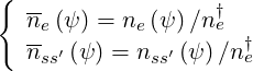 | (6.37) |
and in order to ensure that all quantities are less than unity from the plasma center to the edge, references values are given by the condition
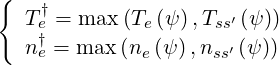 | (6.38) |
for 0 ≤ ψ ≤ ψmax.
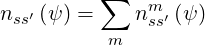
In principle, ion densities nss′ are obtained from a particle transport code
transport code. However, when the plasma is made of two types of ions which are
fully ionized (low Z limit), a simple model may be used in order to determine
densities ns
are obtained from a particle transport code
transport code. However, when the plasma is made of two types of ions which are
fully ionized (low Z limit), a simple model may be used in order to determine
densities ns with s =
  , knowing electron density ne
 and effective
charge Zeff
and effective
charge Zeff profiles. Using the standard definition of Zeff as defined in Ref.
[?]8,
profiles. Using the standard definition of Zeff as defined in Ref.
[?]8,
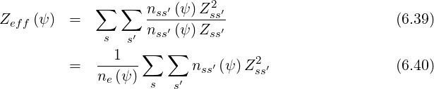
 = ∑
s ∑
s′nss′
= ∑
s ∑
s′nss′ Zss′, one obtains in
this simple case a system of two equations with two unknowns,
Zss′, one obtains in
this simple case a system of two equations with two unknowns,
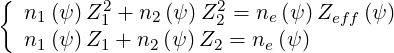 | (6.41) |
Therefore,
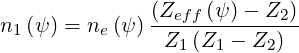 | (6.42) |
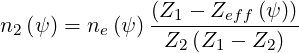 | (6.43) |
and using the normalization rule,
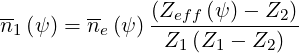 | (6.44) |
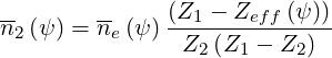 | (6.45) |
since by definition Zeff has no units.
In the calculations, one may also consider several isotopes, since ion inertia play a significant role for the collision operator. Hence,
 | (6.46) |
or
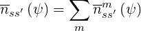 | (6.47) |
where the masses of isotope m of ion species ss′ are mss′m. In the calculations
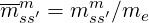 | (6.48) |
where me is the electron rest mass.
The electron-electron Coulomb logarithm lnΛee is defined as the logarithm of the ratio of the maximum to the minimum impact parameters of the Coulomb collision, Λee = bmax∕bmin. Due to screening effect at long distance, bmax = λD, where λD is the Debye length, while bmin is of the order of the Landau scattering length, as discussed in Ref. [?]. Therefore
![[ -3]
lnΛee(ψ ) = 31.3- 0.5 log(ne (ψ ) m )+ log(Te(ψ)[eV ])](NoticeDKE4089x.png) | (6.49) |
and
![† †[ -3] †
lnΛee = 31.3- 0.5log(ne m )+ log(Te [eV ])](NoticeDKE4090x.png) | (6.50) |
Regarding time ordering which is considered in the derivation of the drift kinetic equation and the dominant role played by collisions for the electron momentum distribution function build-up, it is natural to scale time evolution to a reference electron-electron collision frequency νe† according to the relation
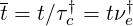 | (6.51) |
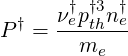
There is arbitrariness in the choice of νe†, since one can use different definition. The relativistic electron-electron collision frequency is used in the code as given in Ref. [?], instead of the usual thermal one discussed in Ref.[?] and Ref.[?] , since its expression is more simple9,
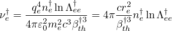 | (6.52) |
Here ε0 = 8.854187818 × 10⁻¹²  is the free space permeability, c = 299792458
 the speed of light, qe = -1.60217733 × 10⁻¹⁹
  the electric charge of the
electron, me = 9.1093897 × 10⁻³¹
the electric charge of the
electron, me = 9.1093897 × 10⁻³¹  the electron rest mass, and lnΛee† is the
usual reference electron-electron thermal Coulomb logarithm [?] taken at Te† and ne†
with
the electron rest mass, and lnΛee† is the
usual reference electron-electron thermal Coulomb logarithm [?] taken at Te† and ne†
with
 | (6.53) |
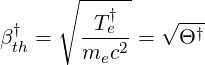
where mec2 = 510.99905  is the electron rest mass energy. In expression 6.52, the classical
electron radius re has been introduced, which is given by
is the electron rest mass energy. In expression 6.52, the classical
electron radius re has been introduced, which is given by
 | (6.54) |
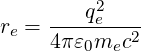
In the calculations, the momentum p in relativistic units  is normalized to the thermal
reference value pth† = mevth†,
is normalized to the thermal
reference value pth† = mevth†,
 | (6.55) |
and consequently
 | (6.56) |
since thermal electrons are only weakly relativistic. The well known relativistic Lorentz correction factor γ is then simply given by the relation
 | (6.57) |
and in the non-relativistic limit, i.e. when p2βth†2 ≪ 1, γ ≈ 1.
Since in relativistic units, the total energy is linked to the relativistic momentum according to the expression,
 | (6.58) |
it is straightforward to expression the kinetic energy Ec as a function of p in units of electron rest mass energy mec2
 | (6.59) |
Finally, concerning the normalization of the electron velocity v, one has
 | (6.61) |
or
 | (6.62) |
with
 | (6.63) |
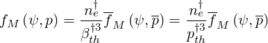
The relativistic Maxwellian fM used in the calculations has the following dependence in p
![[ p2 ] [ γ - 1]
fM (ψ, p) ∝ α exp - --------- = α exp - -----
(1 + γ)Θ Θ](NoticeDKE4112x.png) | (6.64) |
where Θ = Te ∕mec2 and γ2 = p2 + 1. By definition, fM is normalized to the local density
ne
∕mec2 and γ2 = p2 + 1. By definition, fM is normalized to the local density
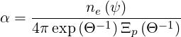
ne , and the parameter α is then given by the integral
![∫ ∞ [ ]
4πα p2exp - γ --1 dp = ne(ψ )
0 Θ](NoticeDKE4115x.png) | (6.65) |
Recalling that γdγ = pdp,
 | (6.66) |
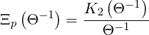
where
![( ) ∫ ∞ ∘ ------ [ ]
Ξp Θ-1 = γ γ2 - 1 exp - γΘ- 1 dγ
1](NoticeDKE4117x.png) | (6.67) |
By integrating by parts,
![( ) - 1∫ ∞ ( ) [ ]
Ξp Θ -1 = Θ--- γ2 - 1 3∕2 exp - γΘ -1 dγ
3 1 ( )
4(3∕2)!K2 Θ -1
= 3-√-π----Θ--1--- (6.68)](NoticeDKE4118x.png)
 ! =
! = 
 !!∕2n
and n!! = 1.3.....n for positive odd n values,
one obtains readily
!!∕2n
and n!! = 1.3.....n for positive odd n values,
one obtains readily
 | (6.69) |
and finally
![ne(ψ ) [ γ - 1 ]
fM (ψ,p) = -----------1--------1-exp - -----
4πΘ exp(Θ )K2 ([Θ )] Θ
= ---ne-(ψ-)----exp - γ- (6.70)
4πΘK2 (Θ -1) Θ](NoticeDKE4123x.png)
For Θ ≪ 1, using the large argument asymptotic development of
K2 ≈
≈
 exp(-Θ-1) + O
 , the usual expression
![[ ]
-ne-(ψ)- γ---1
fM (ψ, p) ≃ [2πΘ ]3∕2 exp - Θ
[ 2 ]
= -ne-(ψ)-exp - ---p----- (6.71)
[2πΘ ]3∕2 (1+ γ) Θ](NoticeDKE4128x.png)
 | (6.72) |
must be fulfiled. Since p may be as large as 30 in calculations, in order to correctly describe momentum dynamics of the fastest electrons, it results that
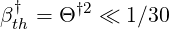 | (6.73) |
or
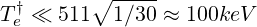 | (6.74) |
Usually, this condition is well satisfied even in the core of tokamak plasmas, where Te† never exceeds 20keV. In normalized units,
![[ ]
ne(ψ)n †e p2β†2
fM (ψ, p) = ---------3∕2-exp - ---------th----†2
[2πΘ (ψ)] (1 + γ)T e(ψ)βth
ne(ψ )n†e [ p2 ]
= [-----------]3∕2 exp - ------------- (6.75)
2πT e(ψ)β †2th (1+ γ )Te(ψ )](NoticeDKE4132x.png)
 . Then, it turns out that
 | (6.76) |
since pth† = βth†, with
![-- ne(ψ ) [ p2 ]
fM (ψ, p) ≈ [--------]3∕2 exp - -------------
2π Te(ψ ) (1+ γ )Te(ψ )](NoticeDKE4135x.png) | (6.77) |
which may be expressed in an alternative form, useful for calculating interpolation between full and half-grids,
![[ ]
-- ne(ψ) γ - 1
fM (ψ,p) ≈ [--------]3∕2 exp - -------†2-
2πT e(ψ) Te(ψ )βth](NoticeDKE4136x.png) | (6.78) |
One can then cross-check that
 | (6.79) |
the local density is well recovered.
For the poloidal flux coordinate, the normalized value is
 | (6.80) |
where ψa is the value at the plasma edge, corresponding usually to the last closed magnetic flux surface, as given by the equilibrium code. Usually, it is taken so that 0 ≤ψ ≤ 1 from the center to the plasma edge. For
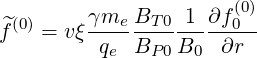
The first order drift kinetic equation requires to calculate 
 defined as
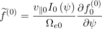 | (6.81) |
where by definition BT0 =
=  ∕R0 and Ωe0 = -
 is the electron Larmor frequency,
all quantities being determined at the poloidal location where the magnetic field B is minimum,
as discussed in Sec. 3.5.5. Since
is the electron Larmor frequency,
all quantities being determined at the poloidal location where the magnetic field B is minimum,
as discussed in Sec. 3.5.5. Since
 | (6.82) |
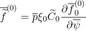
one obtains in normalized units

Therefore,
 | (6.84) |
where
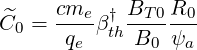 | (6.85) |
For circular concentric flux surfaces, since ∂∕∂ψ =  ∂∕∂r and ∇ψ = RBP , it turns
out that
∂∕∂r and ∇ψ = RBP , it turns
out that
 | (6.86) |
and naturaly
 | (6.87) |
where the safety factor q is approximated by its cylindrical expression q =  , ap the plasma
minor radius, and ϵ = r∕Rp the inverse aspect ratio.
, ap the plasma
minor radius, and ϵ = r∕Rp the inverse aspect ratio.
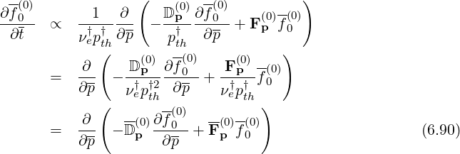
From the conservative form of the Fokker-Planck equation in momentum space
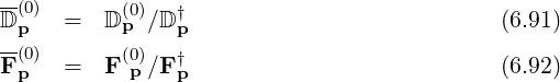
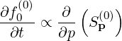 | (6.88) |
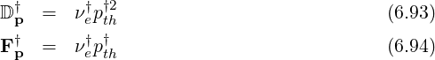
where
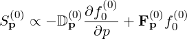 | (6.89) |
Introducing normalized coordinates, it turns out that
For the case of the Ohmic electric field, this normalization leads to introduce naturaly the Dreicer field
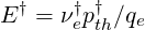 | (6.95) |
the electric field being normalized according to the relation
 | (6.96) |
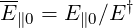
From the conservative form of the Fokker-Planck equation in configuration space
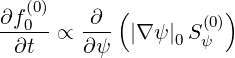 | (6.97) |
where
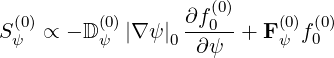 | (6.98) |
Introducing normalized coordinates, it turns out that
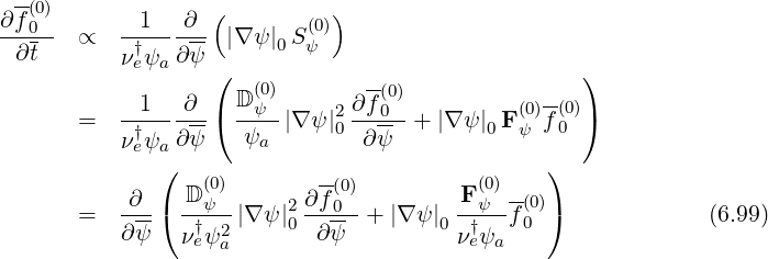
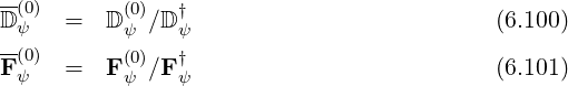
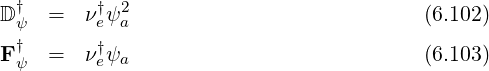
However, since it is more convenient to handle diffusion and convection coefficients that scale in m2∕s and m∕s respectively, one must introduce new reference values for the diffusion and convection coefficients. Let
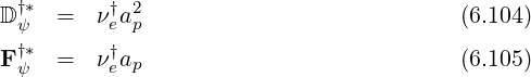
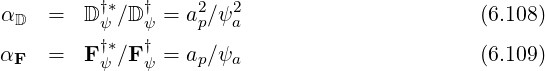
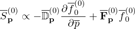
In momentum space,
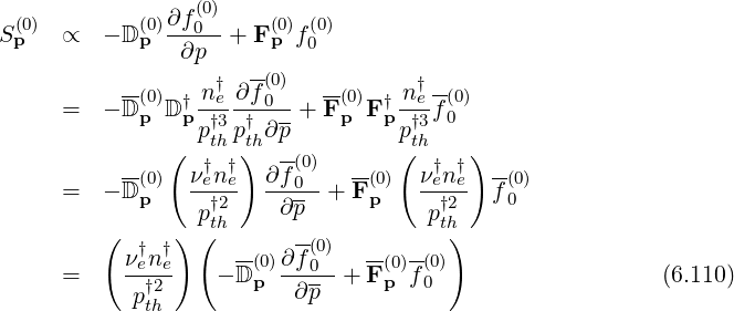
 | (6.111) |
where
 | (6.112) |
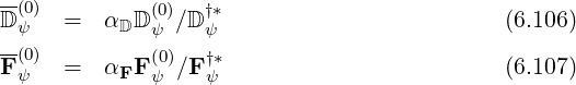
and with these definitions,
 |
A similar procedure is applied for dynamics in configuration space,
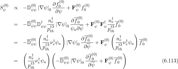
 | (6.114) |
with
 | (6.115) |
and with these definitions,
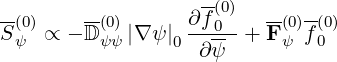 | (6.116) |
The local current density at the minimum B value on the flux surface is given by the relation
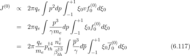
 | (6.118) |
where
 | (6.119) |
With this definition
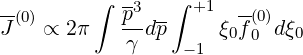 | (6.120) |
The power density is deduced from the integral
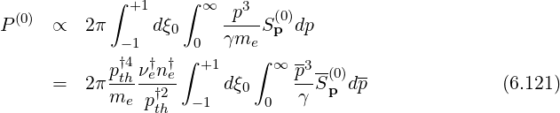
 | (6.122) |
one has
 | (6.123) |
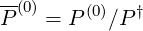
With this definition
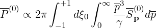 | (6.124) |
The electron runaway rate ΓR is given by the relation
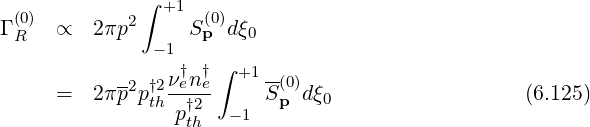
Therefore, normalized expression is
 | (6.126) |
with
 | (6.127) |
so that
 | (6.128) |
The consistency of the normalized units may be benchmarked by the approximate relation
between the total current and the bulk current, the difference coming from the electron runaway
tail. For small ΓR, the runaway distribution is independent of v∥, so that it may be
approximated by the simple expression f0
 ≈
≈ δ
δ . By integrating the
current integral v∥f0
. By integrating the
current integral v∥f0 out to pmax, one obtains
 | (6.129) |
and in normalized units,
 | (6.130) |
so that
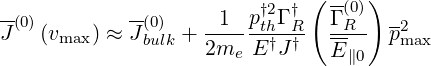 | (6.131) |
According to their respective expression,
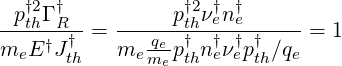 | (6.132) |
which demonstrates the overall consistency of the normalization of the different quantities calculated by the code.
The bounce-averaged avalanche source term  R
R given by relation 3.418, is simply
proportional to
given by relation 3.418, is simply
proportional to  V νe∕lnΛee. Therefore
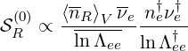 | (6.133) |
where lnΛee = lnΛee∕lnΛee†, and the ratio is
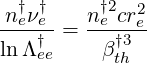 | (6.134) |
By definition, the electron magnetic ripple loss rate ΓST  is given by a relation relation similar
to ΓR
is given by a relation relation similar
to ΓR , except that integrals of fluxes are calculated for different boundaries. Therefore, the
normalized expression is simply given by the relation
, except that integrals of fluxes are calculated for different boundaries. Therefore, the
normalized expression is simply given by the relation
 | (6.135) |
where
 | (6.136) |
In the code, the following units are used
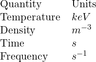 |