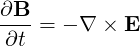
The generation of Ohmic current is based on the concept of transformer, where the plasma torus is the secondary circuit. An electric field is induced by the temporal variation ∂ψ∕∂t of the poloidal flux generated by the primary circuit. The induced current density is then calculated by Ohm’s law, J = σΩE, where σΩ is the electric conductivity calculated by accounting for the Coulomb interaction between the strongly magnetized components of the plasma. Using Faraday’s law,
We consider the surface S which is a truncated cone delimited by two circles being C1,
the magnetic axis, and C2
which is a truncated cone delimited by two circles being C1,
the magnetic axis, and C2 , the toroidal line at position
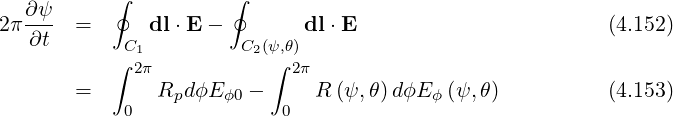
  . Applying the integral
formula to Faraday’s law, we have
. Applying the integral
formula to Faraday’s law, we have
 | (4.150) |
The poloidal flux is given by
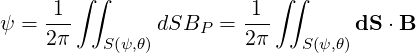 | (4.151) |
so that we get
 | (4.154) |
and therefore
 | (4.155) |
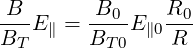
and REϕ is only a function of ψ. We can therefore rewrite
 | (4.156) |
where R0 is the major radius taken at the the poloidal position θ0 where the magnetic field B is minimum on a flux-surface.By definition,
 | (4.157) |
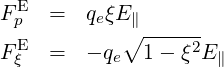
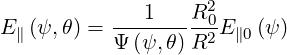
The electric field along the field line can then be obtained by projection, which gives
 | (4.158) |
so that we get
 | (4.159) |
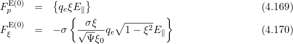
and then
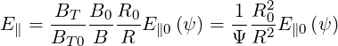 | (4.160) |
with Ψ = B∕B0 as defined in Sec. 2.2.1.
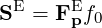
The effect of the electric fied E∥ can be expressed in a conservative form as  (f0) = ∇p ⋅ SE,
where the flux in momentum space is easily expressed in cylindrical coordinates
(f0) = ∇p ⋅ SE,
where the flux in momentum space is easily expressed in cylindrical coordinates  as
as
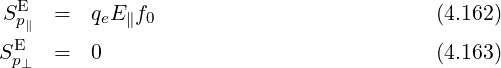
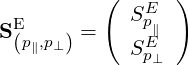 | (4.161) |
with
The transformation from cylindrical to spherical coordinates is given by
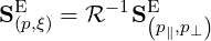 | (4.164) |
where  is the rotational matrix
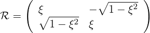
Using -1 = t we find
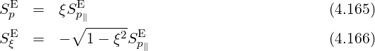
 | (4.167) |
with
In the Fokker-Planck equation, the diffusion and convection elements are bounce-averaged according to the expressions (3.189)-(3.194), which gives, using (4.167),
 | (4.168) |
and the convection components
Since the poloidal dependence of the electric field on a flux-surface is given by ()
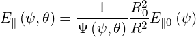 | (4.171) |
we find
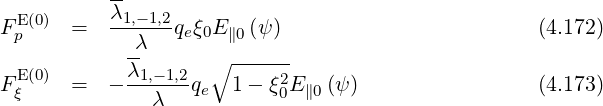
 | (4.174) |
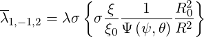
The coefficient λ1,-1,2, which is known as s* in the old notation found in the litterature ([?]), is expressed as
![[ ]
-- σ 1∑ ∫ θmaxdθ 1 r B 1 R2
λ1,-1,2 = -- -- ---||----||------σ------- -02-
q^ 2 σ T θmin 2π |^ψ ⋅^r|Rp BP Ψ (ψ, θ)R](NoticeDKE2043x.png) | (4.175) |
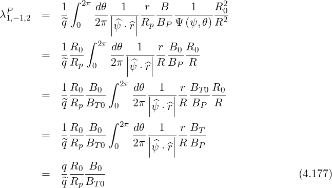
Since the integral is odd in σ, the sum over trapped particles vanishes, and we have
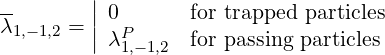 | (4.176) |
Since in the case of circular concentric flux-surfaces, we have
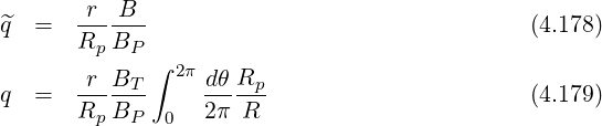
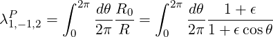 | (4.180) |
This integral can then be performed analytically, as shown in Sec. ??, at formula (??), which gives
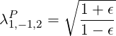 | (4.181) |
In the first order Drift-Kinetic equation, the diffusion and convection flux elements related to  are bounce-averaged according to the expressions (3.218)-(3.223), which gives, using
(4.167),
are bounce-averaged according to the expressions (3.218)-(3.223), which gives, using
(4.167),
 | (4.182) |
and the convection components
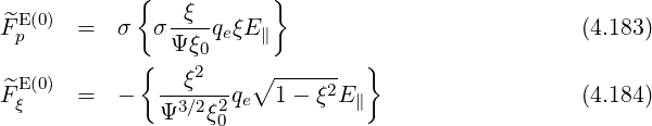
Since the poloidal dependence of the electric field on a flux-surface is given by relation (4.160)
 | (4.185) |
we find
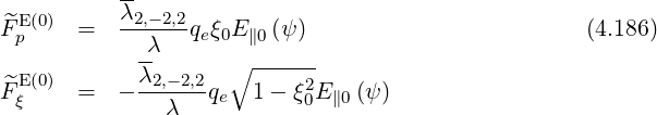
 | (4.187) |