7.5 Fast electron radial transport
This simulation is here presented to illustrate code capabilities for a realistic magnetic
configuration and a hot deuterium plasma. It corresponds to a typical JET Lower Hybrid
current drive discharge, where both bounce-averaging and fast electron particle transport are
considered. Global parameters of the discharge are gathered in section “JET” of the tokamak
parameter M-file “ptok_dke_1yp.m”.
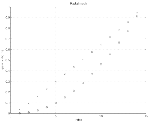
As shown in Fig.7.22 , the spatial ψ half-grid, on which the electron distribution function is
calculated, is non-uniform, though grid steps Δρ for the normalized radius defined in Sec. 2.1
are constant for this example. The spatial mesh size for f0 has nψ - 1 = 14 points,
which is the typical number of spatial grid points considered in most of the current
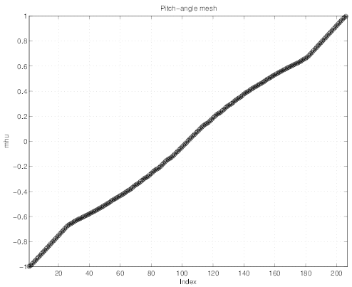
drive simulations. The corresponding pitch-angle grid is strongly non uniform, as
indicated in Fig.7.23, since trapped/passing boundaries corresponding to all radial
positions are exactly placed on the flux grid in momentum space. The total number of
pitch-angle points for f0
has nψ - 1 = 14 points,
which is the typical number of spatial grid points considered in most of the current
drive simulations. The corresponding pitch-angle grid is strongly non uniform, as
indicated in Fig.7.23, since trapped/passing boundaries corresponding to all radial
positions are exactly placed on the flux grid in momentum space. The total number of
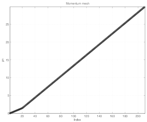
pitch-angle points for f0 is nξ0 - 1 = 206. Finally the momentum grid is also taken no
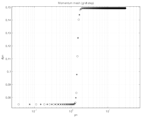
uniform with np - 1 = 210 points. As shown in Fig.7.24 the momentum grid is first
nearly uniform in the vicinity of p = 0 for the first twenty points, with a small step
Δp ≃ 0.07 , as indicated in Fig. 7.25. For p ≳ 1.5, the grid is also uniform, but with larger
momentum step Δp ≃ 0.15. The smooth transition between the two grids involves 7 grid
points.
is nξ0 - 1 = 206. Finally the momentum grid is also taken no
uniform with np - 1 = 210 points. As shown in Fig.7.24 the momentum grid is first
nearly uniform in the vicinity of p = 0 for the first twenty points, with a small step
Δp ≃ 0.07 , as indicated in Fig. 7.25. For p ≳ 1.5, the grid is also uniform, but with larger
momentum step Δp ≃ 0.15. The smooth transition between the two grids involves 7 grid
points.
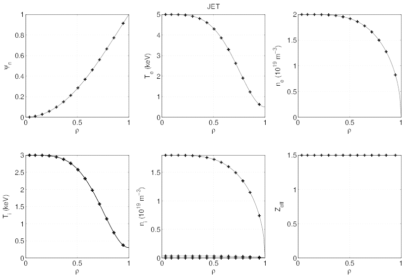
Temperature and density profiles used as input for the magnetic equilibrium calculations
done by HELENA code are presented in Fig. 7.26. As usual in current drive regime at low
density, the electron temperature profile is peaked, and its value is much larger than ion
temperature. The dominant ion (deuterium) profile is determined selfconsistently
from the electron density and effective charge profiles, the latter being taken flat at a
level of Zeff = 1.5. In the calculations which are based on electroneutrality, only
one fully stripped impurity is considered, i.e. carbon Zs = 6, in order to avoid the
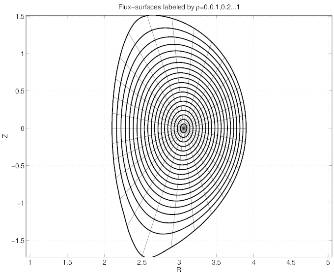
use of an impurity transport code. The resulting 2 - D contour plot of the magnetic
poloidal flux surfaces is given in Fig. 7.27, for a configuration with a bottom X-point
close to the divertor. Here, calculations are performed for a monotonic safety factor
profile.
In the calculations, fully relativistic corrections are considered. In Fig.7.28, the deviation
from the relation v = p clearly indicates that relativistic corrections come into play when
p ≳ 4.
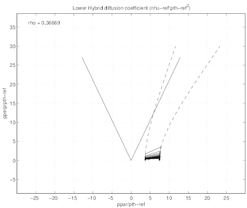
Consequently, since a simplified expression for the Lower Hybrid quasilinear diffusion operator is
considered, as described in Appendix D.2.8 and used in Sec. 7.3, boundary values of the
resonance domain which correspond to  exhibit strong curvature as a
function of p, as shown in Fig. 7.29. In order to simulate a spatialy localized off-axis
absorption of the RF power, the quasilinear diffusion coefficient D0,newLH
exhibit strong curvature as a
function of p, as shown in Fig. 7.29. In order to simulate a spatialy localized off-axis
absorption of the RF power, the quasilinear diffusion coefficient D0,newLH is defined
as
is defined
as
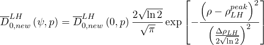 | (7.12) |
where D0,newLH = 1 in the interval v1 ≤ v∥≤ v2, and ρLHpeak = 0.5 is the radial position
at which absorption is maximum, and ΔρLH = 0.2 the half-width. For ρ ≤ 0.2 and ρ ≥ 0.65,
power absorption is null.
= 1 in the interval v1 ≤ v∥≤ v2, and ρLHpeak = 0.5 is the radial position
at which absorption is maximum, and ΔρLH = 0.2 the half-width. For ρ ≤ 0.2 and ρ ≥ 0.65,
power absorption is null.
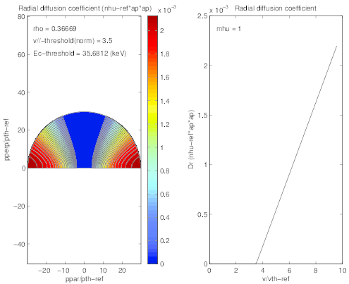
Fast electron radial transport that could result from magnetic turbulence is expressed in the
usual form
 | (7.13) |
where Dψ is the radial diffusion coefficient as defined in Sec.6.3. Here, Dψ
 scales like
  as
expected from theory [?], with a velocity threshold which is set to 3.5. The simulation is
performed with Dψ
as
expected from theory [?], with a velocity threshold which is set to 3.5. The simulation is
performed with Dψ = 5m2∕s, its value and the threshold level being uniform throughout the
plasma, while any convection is neglected. The 2 -D contour plot of the Dψ
= 5m2∕s, its value and the threshold level being uniform throughout the
plasma, while any convection is neglected. The 2 -D contour plot of the Dψ is shown in Fig.
7.30
is shown in Fig.
7.30
The 3 - D simulation is performed in the fully implicit mode with usual parameters,
i.e. Δt = 10000, using the linearized electron-electron Belaiev-Budker collision
operator for momentum conservation. While the time taken to calculate all matrix
coefficients associated to momentum dynamics is extremely fast, of the order of
120s,
since calculations may be performed in a vectorial form that is very convenient for MatLab,
coefficients for radial transport needs a much longer computer time is this version of the code,
typically an order of magnitude more. This limitation results from the fact that loops have been
used in MatLab as a consequence of the complexity of the coefficients arrangement in the matrix
related to the change of the trapped/passing boundary with radial position. In that case, a
specific MEX-file written in C or FORTRAN should considerably reduce time consumption, at a
level comparable to the one needed for calculating the coefficients which result from momentum
dynamics.
In the case of full 3 - D calculation, the Maxwellian solution is imposed at i = 1∕2.
Though this condition is not necessary in principle, it turns out to increase matrix
conditionning, and reduce significantly the memory required to store LU matrices. However,
no normalization of the density at each time step is performed. Consequently, the
drop tolerance for incomplete LU matrix factorization may be increased from 10-4 to
10-3 as compared to the case without radial transport, a important advantage since
it reduces considerably computer time consumption for performing the incomplete
factorization.
On a Compaq workstation, the characteristic time used for this calculation is around 1500s,
and the memory required to store LU matrices is 214MBytes in the example here
studied.
Once LU matrices are calculated, the convergence is very fast. it is achieved after 6
iterations, corresponding to the minimum value required for a correct convergence with the
explicit momentum conservation term (first Legendre truncated term) as discussed
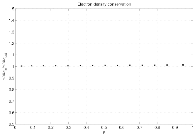
in Sec.6.2.2. As shown in Fig.7.31, the code is fully conservative, within less than
1%.
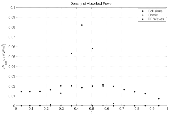
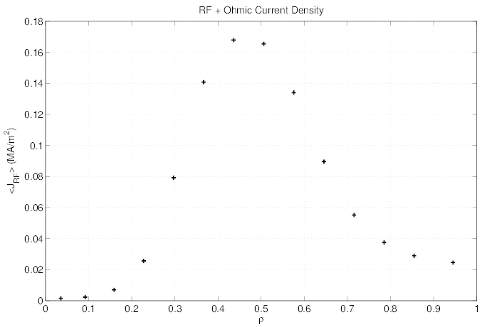
While the absorbed RF power density profile given in Fig.7.32 shows a localized
peak around ρ = 0.5, the current density profile is much broader, as indicated in
Fig.7.33. In the direction of the plasma center, the broadening effect is weak, since
collisional slowing down prevails over radial transport when density is high. Towards
plasma edge, the effect of radial transport is much more visible, and for ρ ≥ 0.6, all the
fast electrons are driven by this mechanism instead of direct kinetic resonance. The
effect of plasma magnetic equibrium on radial transport is fully considered in the
calculations.
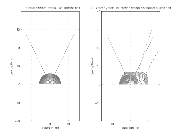
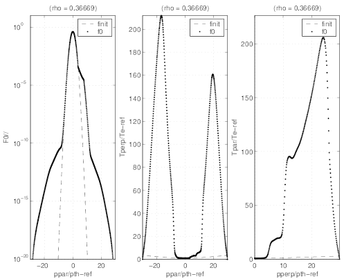
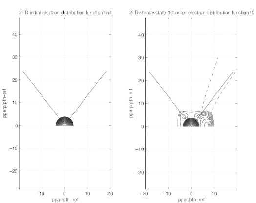
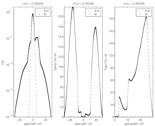
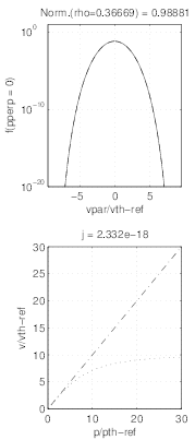
Comparison between distributions at radial positions where RF absorption peaks (Figs.7.34
and 7.35) and in the region where radial transport predominates (Figs.7.36 and 7.37) clearly
shows the difference of dynamics in momentum space. While a plateau is clearly formed at
ρ ≃ 0.36, the distribution exibits a bump at ρ ≃ 0.78. There are nevertheless some
reminiscence of the Lower Hybrid quasilinear resonance boundaries. In all figures, the
output of the code is clean from numerical instabilities, even far from the resonance
domain, which confirms the robustness of the numerical scheme here employed for 3 - D
calculations.
Finally, it is important to mention that the power density absorbed by collisions is much
broader than the RF contribution, as shown in Fig. 7.32. Since radial fast electron transport
makes the current response non-local, in that case the current drive efficiency may be only
defined as the ratio of the total current driven by the wave and the total RF absorbed power in
the plasma.
 at
at