 (0) defined as
Spatial grid interpolation for gradient calculation
The first order drift kinetic equation requires to calculate (0) defined as
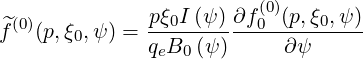 | (5.315) |
where  = RBT . Here all quantities are determined on the poloidal position where the
magnetic field B is minimum.
= RBT . Here all quantities are determined on the poloidal position where the
magnetic field B is minimum.
The spatial grid being non-uniform, radial derivative requires a specific treatment, for an accurate determination. Let ψ-,ψ et ψ+ the three neighbor radial positions where are calculated the distribution function f0(0) with Δψ- = ψ-- ψ, Δψ+ = ψ+ - ψ and Δψ = ψ+ - ψ-. A parabolic interpolation of the form y = aψ2 + bψ + c is used for calculating the radial derivative dy∕dψ = 2aψ + b. The coefficients a,b and c being determined by values y-,y and y+ at grid points ψ-,ψ and ψ+, one can easily show that
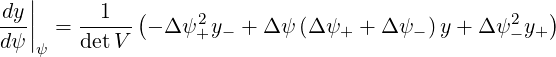 | (5.316) |
where V is a Van der Monde matrix of order 3,
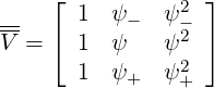 | (5.317) |
whose determinant is simply
 | (5.318) |
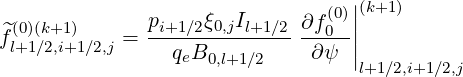
Therefore
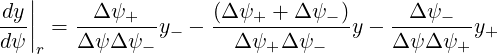 | (5.319) |
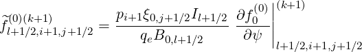
and applying this result for  (0),
(0),
![(0)(k+1) pi+1∕2ξ0,j+1∕2Il+1∕2
f^l+1∕2,i+1∕2,j+1∕2 = -----qB-----------×
[ ( e )0,l+1∕2
---------ψl+3∕2 --ψl+1∕2-------- (0)(k+1)
(ψ - ψ )(ψ - ψ )f0,l-1∕2,i+1 ∕2,j+1∕2
l+3(∕2 l-1∕2 l-1∕2 l+1)∕2
-----ψl+3∕2---2ψl+1∕2 +-ψl-1∕2--- (0)(k+1)
- (ψ - ψ )(ψ - ψ )f0,l+1∕2,i+1∕2,j+1∕2
l+3∕2 ( l+1∕2 l-1∕2 ) l+1∕2 ]
---------ψl-1∕2 --ψl+1∕2-------- (0)(k+1)
- (ψ - ψ )(ψ - ψ )f0,l+3∕2,i+1∕2,j+1∕2 (5.320)
l+3∕2 l-1∕2 l+3∕2 l+1∕2](NoticeDKE3279x.png)
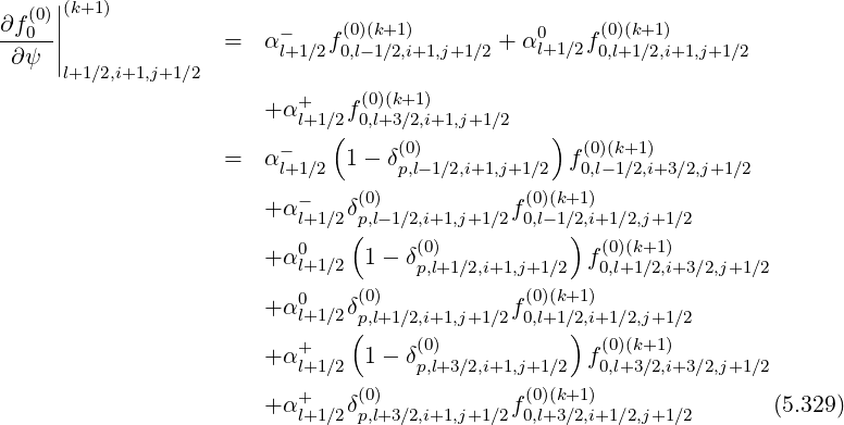
 . In a compact form,
 ![(0)(k+1) pi+1∕2ξ0,j+1∕2Il+1∕2
^fl+1∕2,i+1∕2,j+1∕2 =-----qB-----------×
[ e 0,l+1∕2
α- f(0)(k+1) + α0l+1∕2f (0)(k+1)
l+1∕2 0,l-1∕2,i+1∕2,j+1∕2 ] 0,l+1∕2,i+1∕2,j+1∕2
+α+l+1∕2f(00,l)(+k3+∕12),i+1∕2,j+1∕2 (5.321)](NoticeDKE3281x.png)
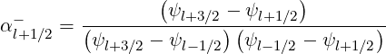 | (5.322) |
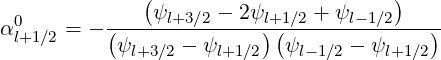 | (5.323) |
and
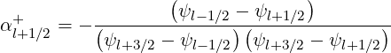 | (5.324) |
Momentum grid interpolation
As indicated in Sec. 3.5.5, it is possible to keep the conservative form for the first-order drift
kinetic equation. The main advantage is that the numerical differencing technique
already used for the zero-order Fokker-Planck equation may be also employed for
determining the numerical solution of this equation. The determination of the momentum
 l+1∕2,i+1∕2,j+1∕2(k) and pitch-angle
  l+1∕2,i+1∕2,j+1∕2(k) derivatives
requires, as for f0
l+1∕2,i+1∕2,j+1∕2(k) derivatives
requires, as for f0 , interpolation techniques in order to evaluate
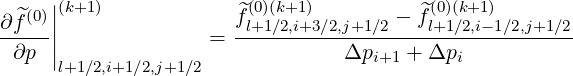
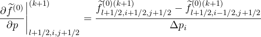
  (0) on flux grid at the
radial position l + 1∕2. By analogy, one have to determine
(0) on flux grid at the
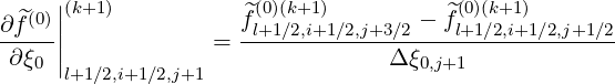
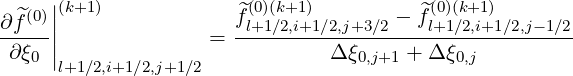
radial position l + 1∕2. By analogy, one have to determine  (0) on the following grid
points
(0) on the following grid
points
 | (5.325) |
 | (5.326) |
 | (5.327) |
and
 | (5.328) |
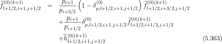
Using the weighting factors δp(0) introduced for f0 , as shown in Sec. 5.4.3 which both are
functions of ψ, one obtains for the grid point
, as shown in Sec. 5.4.3 which both are
functions of ψ, one obtains for the grid point 
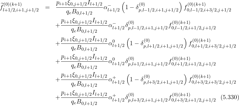
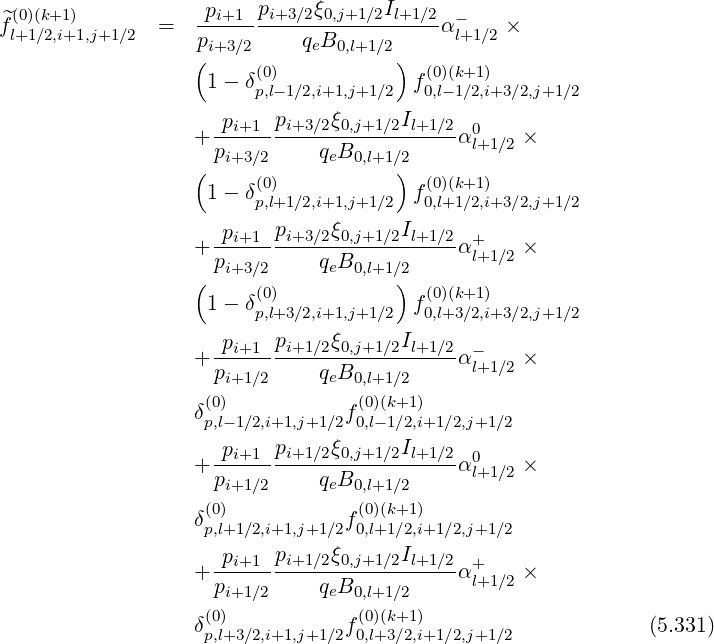

Reordering coefficients, one obtains,
This double difference makes coefficient  l+1∕2,i+1,j+1∕2
 is second order correction, that is
almost negligible when spatial gradients are weak. However, for strong gradients, this correction
must be, in principle, considered.
is second order correction, that is
almost negligible when spatial gradients are weak. However, for strong gradients, this correction
must be, in principle, considered.
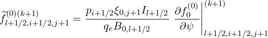
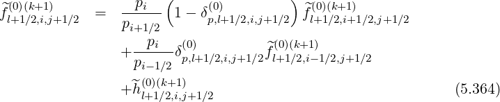
A similar expression is obtained for the grid point 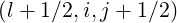 , by replacing i + 1 → i
in all above relations.
, by replacing i + 1 → i
in all above relations.
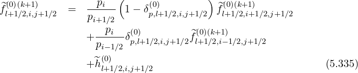
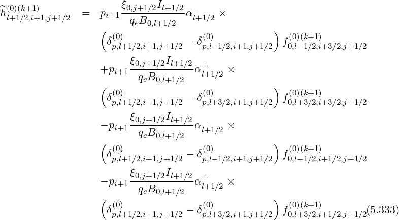
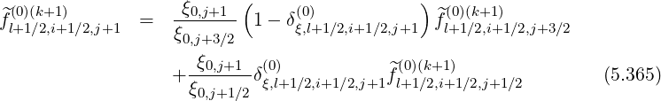
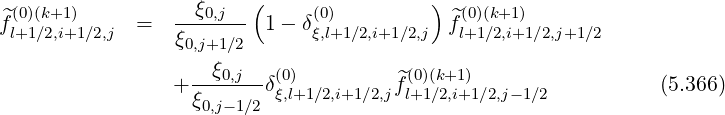
Finally, a similar approach may be used for the pitch-angle grid interpolation. For grid points
 ,
,
![(0)(k+1) ξ0,j+1Il+1∕2
^hl+1∕2,i+1 ∕2,j+1 = pi+1∕2 q-B--------×
[ e( 0,l+1∕2 )
α-l+1∕2 δ(ξ0,l)+1∕2,i+1 ∕2,j+1 - δ(ξ0,l)-1∕2,i+1∕2,j+1 ×
( )
f(00,l)(-k1+∕12),i+1∕2,j+3∕2 - f(00,l)(-k1+∕12,)i+1∕2,j+1∕2
( )
+ α+l+1∕2 δ(0ξ,)l+1∕2,i+1∕2,j+1 - δ(0ξ,)l+3∕2,i+1∕2,j+1 ×
( )]
f0(0,)l+(k3+∕12),i+1∕2,j+3∕2 - f(00,l)(+k3+∕12),i+1∕2,j+1 ∕2 (5.338)](NoticeDKE3309x.png)
However, since by definition, δξ,l+1∕2,i+1∕2,j+1(0) = δξ,l-1∕2,i+1∕2,j+1(0), and δξ,l+1∕2,i+1∕2,j+1(0) = δξ,l+3∕2,i+1∕2,j+1(0), it turns out that
 | (5.339) |
and a similar result is obtained for grid points 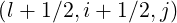 , expressions are
 | (5.341) |
The starting point of the discrete representation of the first order drift kinetic equation is the conservative relation
 and Sξ
 are fluxes related to the function g
 as introduced in Sec.3.5.5, while
 p
p and
and  ξ
ξ are fluxes related to the function
 . Since g
 and f0
 have same symmetries
with respect to the pitch-angle ξ0, matrix coefficients are exactly identical for both
functions (see Sec. 5.4.1). However, calculations are slightly different for
have same symmetries
with respect to the pitch-angle ξ0, matrix coefficients are exactly identical for both
functions (see Sec. 5.4.1). However, calculations are slightly different for 
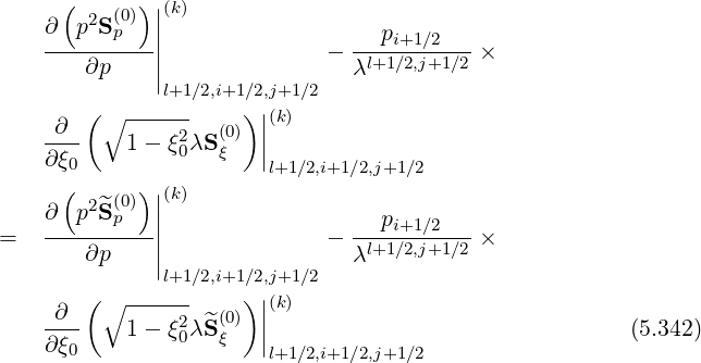
 , though a
conservative form may still be kept. By analogy with zero order Fokker-Planck equation,
, though a
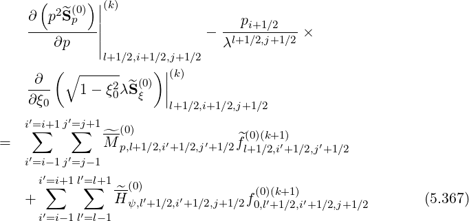
conservative form may still be kept. By analogy with zero order Fokker-Planck equation,
![( 2 (0))||(k)
∂--p-^Sp---|| ---pi+1-∕2---
∂p | - λl+1∕2,j+1∕2 ×
|l+1∕2,i+1∕2,j+1∕2
(∘ ------ )||(k)
-∂-- 1- ξ20λ^S (0) |
∂ ξ0 ξ |l+1 ∕2,i+1∕2,j+1∕2
m∑=8
= ^T[m] (5.345)
m=1](NoticeDKE3330x.png)
![2 ^(0) ∂^f(0)||(k+1) 2 ^(0) ^(0)(k+1)
[1] - pi+1D-pp,l+1∕2,i+1,j+1∕2-∂p-|l+1∕2,i+1,j+1∕2 +-p-i+1F-p,l+1∕2,i+1,j+1∕2fl+1∕2,i+1,j+1∕2
T^ = Δp
i+1∕2](NoticeDKE3331x.png) | (5.346) |
![(0) ∂^f(0)||(k+1 ) (0) (0)(k+1)
p2iD ^pp,l+1∕2,i,j+1∕2-∂p-| - p2i ^Fp,l+1∕2,i,j+1∕2f^l+1∕2,i,j+1∕2
T^[2] =----------------------l+1∕2,i,j+1∕2-----------------------------
Δpi+1∕2](NoticeDKE3332x.png) | (5.347) |
![( )| |
∘ -----------∂ p^Dp(0ξ) || ∂ ^f(0)|(k+1)
^T [3] = + 1- ξ20,j+1∕2 ---------|| ----||
∂p | ∂ξ |l+1∕2,i+1∕2,j+1∕2
l+1∕2,i+1∕2,j+1∕2](NoticeDKE3333x.png) | (5.348) |
![∘ ----------- 2 (0)||(k+1)
T^[4] = + 1 - ξ2 p ^D (0) ∂-f^--||
0,j+1∕2 i+1∕2 pξ,l+1∕2,i+1∕2,j+1∕2 ∂p∂ξ |
l+1∕2,i+1∕2,j+1∕2](NoticeDKE3334x.png) | (5.349) |
![⌊ (0) ( 2 ) l+1∕2,j+1 ∂^f(0)||(k+1)
pi+1∕2 | ^Dξξ,l+1∕2,i+1∕2,j+1 1 - ξ0,j+1 λ -∂ξ-|l+1∕2,i+1∕2,j+1
T^[5] = - -l+1∕2,j+1∕2-|⌈ -------------------------------------------------------
λ pi+1∕2Δ ξj+1∕2
∘ --------- ⌋
pi+1∕2 1- ξ2 λl+1∕2,j+1F^(0) f^(0)(k+1)
+ -----------0,j+1-----------ξ,l+1-∕2,i+1∕2,j+1-l+1∕2,i+1∕2,j+1-⌉ (5.350)
Δ ξj+1∕2](NoticeDKE3335x.png)
![⌊
^ (0) ( 2 ) l+1∕2,j ∂^f(0)||(k+1)
[6] pi+1∕2 | D ξξ,l+1∕2,i+1∕2,j 1 - ξ0,j λ ∂ξ |l+1∕2,i+1∕2,j
T^ = λl+1∕2,j+1∕2|⌈ -----------------p----Δ-ξ----------------------
i+1∕2 j+1∕2
∘ ------- ⌋
pi+1∕2 1- ξ02,jλl+1∕2,jF^(0) ^f(0)(k+1)
+ -----------------------ξ,l+1∕2,i+1∕2,j-l+1-∕2,i+1∕2,j⌉ (5.351)
Δ ξj+1∕2](NoticeDKE3336x.png)
![p (∘ ------ ) || ^(0)||(k+1)
^T[7] = ---i+1∕2----∂-- 1 - ξ20λD^(ξ0)p | ∂f---||
λl+1∕2,j+1∕2 ∂ξ0 |l+1∕2,i+1∕2,j+1 ∕2 ∂p |l+1∕2,i+1∕2,j+1∕2](NoticeDKE3337x.png) | (5.352) |
![p ∘ ----------- ∂2 ^f(0)||(k+1)
T^[8] = ---i+1∕2--- 1 - ξ20,j+1∕2λl+1∕2,j+1∕2 ^D (0ξp),l+1∕2,i+1∕2,j+1∕2-----||
λl+1∕2,j+1∕2 ∂ ξ0∂p|l+1∕2,i+1∕2,j+1∕2](NoticeDKE3338x.png) | (5.353) |
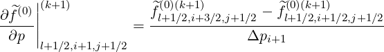
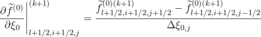
Discrete expressions of the partial derivatives are,
 | (5.354) |
 | (5.355) |
 | (5.356) |
 | (5.357) |
 | (5.358) |
 | (5.359) |
and cross-derivatives
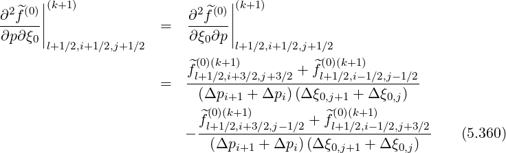
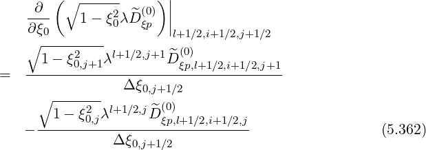
As for the zero-order Fokker-Planck equation, other derivatives in discrete form become
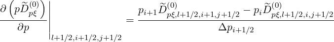 | (5.361) |
Since the distribution function 
 is defined on the half grid, while fluxes on the full grid, it
is necessary to interpolate, because in some derivatives, values of are taken on the full grid. As
discussed in the previous section, interpolation procedure is more complex for
is defined on the half grid, while fluxes on the full grid, it
is necessary to interpolate, because in some derivatives, values of are taken on the full grid. As
discussed in the previous section, interpolation procedure is more complex for 
 than for f0
 .
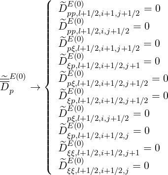
Therefore, for terms proportional to
.
Therefore, for terms proportional to  ξξ
ξξ and
and  ξ
ξ
 ξξ
ξξ and
and  ξ
ξ
 l+1∕2,i+1∕2,j+1
 =
=  l+1∕2,i+1∕2,j
 = 0.
= 0.
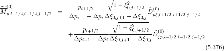
Gathering all terms in a matrix form

 and M
and M have a very similar expressions, though slightly different because of the
ratios pi+1∕pi+3∕2,pi∕pi+1∕2,ξ0,j+1∕ξ0,j+3∕2 and ξ0,j∕ξ0,j+1∕2 but one matrix
have a very similar expressions, though slightly different because of the
ratios pi+1∕pi+3∕2,pi∕pi+1∕2,ξ0,j+1∕ξ0,j+3∕2 and ξ0,j∕ξ0,j+1∕2 but one matrix  ψ
ψ that results
from the spatial variation of the Chang and Cooper coefficients as shown in Sec. 5.4.3. Starting
from the expression of M
that results
from the spatial variation of the Chang and Cooper coefficients as shown in Sec. 5.4.3. Starting
from the expression of M , one obtains
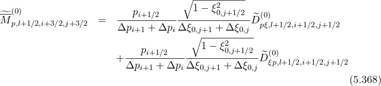
![∘1----ξ2-----
-^-(0) --pi+1----------0,j+1∕2--^(0)
M p,l+1 ∕2,i+1∕2,j+3∕2 = Δpi+1 ∕2Δ ξ0,j+1 + Δ ξ0,jD pξ,l+1∕2,i+1,j+1∕2
∘ -----------
pi 1- ξ20,j+1∕2 (0)
- Δp------Δξ-----+-Δ-ξ--^D pξ,l+1∕2,i,j+1∕2
i+1∕2 0,j+1 0,j
---1---ξ20,j+1-----λl+1∕2,j+1--^(0)
- Δ ξ0,j+1∕2Δξ0,j+1 λl+1∕2,j+1∕2D ξξ,l+1∕2,i+1∕2,j+1
∘ ---------
1- ξ20,j+1 [ ξ ] ( )
- pi+1 ∕2----------- --0,j+1- 1- δ(ξ0,l)+1∕2,i+1∕2,j+1 ×
Δξ0,j+1∕2 ξ0,j+3∕2
λl+1∕2,j+1 (0)
λl+1∕2,j+1∕2 ^Fξ,l+1∕2,i+1∕2,j+1
(5.369)](NoticeDKE3377x.png)

+ --pi+1--- -pi+1-- 1 - δ(0) ^F(0)
Δpi+1∕2 pi+3∕2 p,l+1∕2,i+1,j+1 ∕2 p,l+1∕2,i+1,j+1∕2
(5.371)](NoticeDKE3379x.png)
![^-(0) p2i+1 (0)
M p,i+1∕2,j+1∕2 = Δp-----Δp----^D pp,l+1∕2,i+1,j+1∕2
i+1∕2 i+1 [ ]
-p2i+1--^ pi+1-- (0)
+ Δpi+1∕2Fp,l+1∕2,i+1,j+1∕2 pi+1∕2 δp,l+1∕2,i+1,j+1∕2
2
+ ----pi----D^(0)
Δpi+1∕2Δpi pp,l+1∕2,i,j+1∕2
p2 [ pi ] ( (0) ) (0)
- ---i---- ------ 1- δp,l+1∕2,i,j+1∕2 ^Fp,l+1∕2,i,j+1∕2
Δpi+1∕2 pi+1∕2
1- ξ02,j+1 λl+1∕2,j+1 (0)
- Δξ------Δ-ξ----λl+1∕2,j+1∕2 ^D ξξ,l+1∕2,i+1∕2,j+1
0,j+1∘∕2---0,j+1-
1 - ξ20,j+1[ ξ ]
- pi+1∕2---------- -0,j+1-- δ(ξ0,l)+1∕2,i+1∕2,j+1 ×
Δ ξ0,j+1∕2 ξ0,j+1∕2
λl+1∕2,j+1 (0)
-l+1∕2,j+1∕2 ^Fξ,l+1∕2,i+1∕2,j+1
λ 2 l+1∕2,j
+ ---1---ξ0,j-----λ--------^D (0)
Δξ0,jΔ ξ0,j+1∕2λl+1∕2,j+1∕2 ξξ,l+1∕2,i+1∕2,j
∘ -----2-[ ]
--1---ξ0,j -ξ0,j-- ( (0) )
+pi+1∕2Δ ξ ξ 1 - δξ,l+1 ∕2,i+1∕2,j ×
0,j+1∕2 0,j+1∕2
--λl+1∕2,j--F(0)
λl+1∕2,j+1∕2 ξ,l+1∕2,i+1∕2,j
(5.372)](NoticeDKE3380x.png)
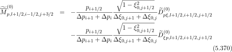
![^-(0) p2i (0)
M p,l+1∕2,i-1∕2,j+1 ∕2 = - Δp-----Δp-D^pp,l+1∕2,i,j+1 ∕2
i+1∕2 i ∘ ---------
p 1- ξ2
- ----i+1∕2----------0,j+1 ×
Δpi+1 + Δpi Δξ0,j+1∕2
λl+1∕2,j+1 (0)
-l+1∕2,j+1-∕2-^Dξp,l+1∕2,i+1 ∕2,j+1
λ ∘ -------
pi+1∕2 1- ξ20,j
+ -------------------- ×
Δpi+1 + Δpi Δξ0,j+1∕2
λl+1 ∕2,j (0)
λl+1∕2,j+1-∕2-^Dξp,l+1∕2,i+1 ∕2,j
2 [ ]
- --pi---- -pi--- δ(0p,)i,j+1∕2F^(p,0)l+1∕2,i,j+1∕2
Δpi+1∕2 pi-1∕2
(5.373)](NoticeDKE3381x.png)
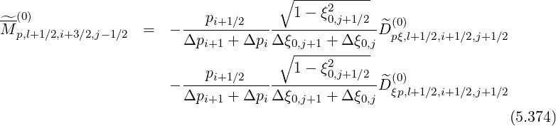
![∘1---ξ2------
^-(0) --pi+1----------0,j+1∕2--^(0)
M p,l+1∕2,i+1∕2,j-1∕2 = - Δpi+1 ∕2 Δ ξ0,j+1 + Δ ξ0,jD pξ,l+1∕2,i+1,j+1∕2
∘ -----------
pi 1- ξ20,j+1∕2 (0)
+ Δp------Δ-ξ----+-Δ-ξ--D^pξ,l+1∕2,i,j+1∕2
i+1∕2 0,j+1 0,j
---1---ξ20,j------λl+1∕2,j--^(0)
- Δ ξ0,j+1∕2Δξ0,jλl+1∕2,j+1 ∕2D ξξ,l+1∕2,i+1∕2,j
∘ -------
1- ξ20,j [ ξ ]
+pi+1 ∕2 --------- ---0,j-- δξ(0,)l+1∕2,i+1∕2,j ×
Δξ0,j+1∕2 ξ0,j-1∕2
λl+1∕2,j (0)
λl+1∕2,j+1∕2F^ξ,l+1∕2,i+1∕2,j
(5.375)](NoticeDKE3383x.png)
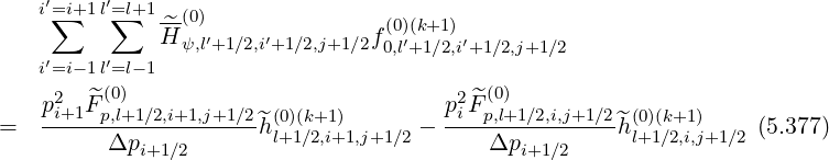
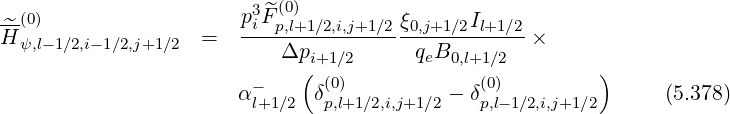
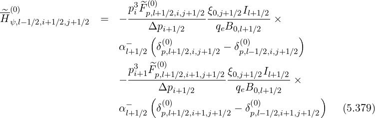
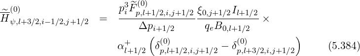
For the determination of matrix  ψ
ψ , it is useful to start from terms
  1 and
1 and  2 that
contain
2 that
contain  l+1∕2,i,j+1∕2
 (k+1) and
  l+1∕2,i+1,j+1∕2
 (k+1). coefficients. Because of the grid
interpolation
(k+1). coefficients. Because of the grid
interpolation
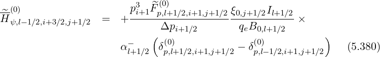
 | (5.381) |
 | (5.382) |
 | (5.383) |
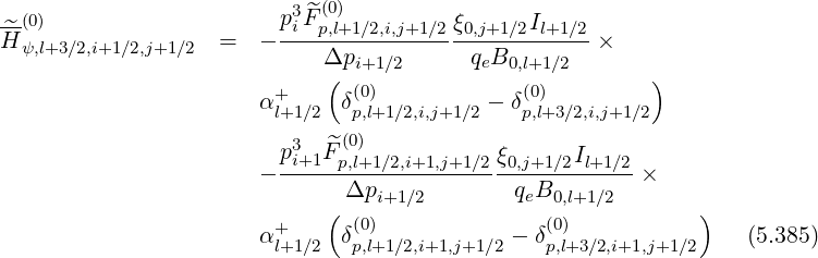
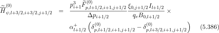
Since first order drift kinetic terms may be expressed in a conservative form as for the zero order Fokker-Planck equation, the determination of the matrix elements is therefore straightforward. One obtains
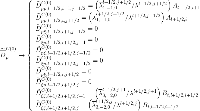 | (5.387) |
and
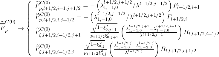 | (5.388) |
where coefficients of the collision operator A,F and Bt are the same as defined for the zero order bounce averaged Fokker-Planck equation, in Sec. 5.4.4.
Concerning the first order Legendre correction for electron-electron collisions that ensures momentum conservation, one must calculate

on the distribution function grid, where
 | (5.389) |
as shwon in Sec. 4.1.7.
Here, the collision integral 
 has a similar form as for the zero order
Fokker-Planck equation except that f0
has a similar form as for the zero order
Fokker-Planck equation except that f0
 is just replaced by
  0
0
 in all corresponding
terms. Therefore, by definition, at the iteration number
in all corresponding
terms. Therefore, by definition, at the iteration number  ,
,
 l+1∕2,i+1∕2,j+1∕2 l+1∕2,i+1∕2,j+1∕2 | = -  H H | ||
× l+1∕2,i+1∕2,j+1∕2 l+1∕2,i+1∕2,j+1∕2 | (5.390) |
where
 | (5.391) |
According to the bounce averaged expression,
 | (5.392) |
and
 | (5.393) |
where E∥0,l+1∕2 is the parallel component of the Ohmic electric field along the magnetic field line direction normalized to the Dreicer field taken at the poloidal position where the magnetic field B is minimum, as explained in Sec.4.2.
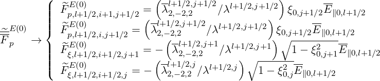
From the expressions given in Sec. 4.3.8, the components of the tensor  pRF
pRF are
are
![^ RF(0) ∑+ ∞ ∑ 2 -^RF(0)D
D pp,l+1∕2,i+1,j+1∕2 = n=-∞ b(1 - ξ0,j+1∕2)D b,n,l+1∕2,i+1,j+1∕2
^DRF (0) = ∑+ ∞ ∑ (1 - ξ2 )D^RF (0)D
pp,l+1∕2,i,j+1∕2 n=-∞ b ∘0,j+1∕2---b,n[,l+1∕2,i,j+1∕2 ]
^DRF (0) = ∑+ ∞ ∑ - -1-ξ20,j+1∕2- 1- ξ2 - nΩ0l+1∕2,i+1-D^RF (0)D
pξ,l+1∕2,i+1,j+1∕2 n=-∞ b ∘ξ0,j+1∕2- 0,j+1∕2 ωb b,n,l+1∕2,i+1,j+1∕2
^ RF(0) ∑+ ∞ ∑ -1-ξ20,j+1[ 2 nΩ0l+1∕2,i+1∕2] ^-RF(0)D
D ξp,l+1∕2,i+1∕2,j+1 = n=-∞ b- ξ∘0,j+1---1-- ξ0,j+1 - ωb D b,n,l+1∕2,i+1∕2,j+1
^ RF(0) ∑+ ∞ ∑ --1-ξ20,j+1∕2[ 2 nΩ0l+1∕2,i+1∕2] ^RF (0)D
D pξ,l+1∕2,i+1∕2,j+1∕2 = n= -∞ b- ∘ ξ0,j+1∕2-- 1 - ξ0,j+1∕2 - ωb Db,n,l+1∕2,i+1∕2,j+1∕2
RF(0) ∑+ ∞ ∑ 1-ξ20,j+1∕2[ 2 nΩ0l+1∕2,i+1∕2] ^RF (0)D
^D ξp,l+1∕2,i+1∕2,j+1∕2 = n= -∞ ∘b----ξ0,j+1∕2-- 1 - ξ0,j+1∕2 ------ωb---- Db,n,l+1∕2,i+1∕2,j+1∕2
RF(0) ∑ ∑ 1-ξ20,j+1∕2[ nΩ ] -RF (0)D
^D pξ,l+1∕2,i,j+1∕2 = +n∞=-∞ b ---ξ0,j+1∕2-- 1 - ξ20,j+1∕2 - --0lω+b1∕2,i- ^Db,n,l+1∕2,i,j+1∕2
∑ ∑ ∘1--ξ2-[ nΩ ]--RF(0)D
^DRFξp,(0l+)1∕2,i+1∕2,j = +n∞=-∞ b ---ξ0,j0,j 1 - ξ20,j - --0l+1ω∕2b,i+1∕2 ^D b,n,l+1∕2,i+1∕2,j
RF(0) ∑ ∑ [ nΩ ]2--RF(0)D
^D ξξ,l+1∕2,i+1∕2,j+1 = +n∞=-∞ b ξ21-- 1- ξ20,j+1 - --0l+1∕ω2b,i+1∕2 D^b,n,l+1∕2,i+1∕2,j+1
RF(0) ∑ ∑ 0,j+1[ nΩ ]2--RF(0)D
^D ξξ,l+1∕2,i+1∕2,j = +n∞=-∞ b ξ21-- 1- ξ20,j+1 - --0l+1∕ω2b,i+1∕2 D^b,n,l+1∕2,i+1∕2,j
0,j+1](NoticeDKE3426x.png) | (5.394) |
and the components of the vector  pRF
pRF are
are
![∘1-ξ20,j+1∕2 ∑ ∑ ∘1-ξ20,j+1∕2 [ nΩ ]--RF(0)F
^FRpF,l+(01)∕2,i+1,j+1∕2 = pi+1ξ3----- +n∞=-∞ b- -ξ0,j+1∕2--- 1- ξ20,j+1∕2 - --0,l+1ω∕b2,i+1 ^D b,n,l+1∕2,i+1,j+1∕2
∘1-ξ2-0,j+1∕2 ∘1-ξ2---- [ ]--RF(0)F
^FRF (0) = ---30,j+1∕2-∑+ ∞ ∑ - ----0,j+1∕2- 1- ξ2 - nΩ0,l+1∕2,i D^b,n,l+1∕2,i,j+1∕2
p,l+1∕2,i,j+1∕2 piξ∘0,j+1∕2--- n=-∞ b ξ0,j+1∕2 0,j+1∕2 ωb
^RF (0) --1--ξ02,j+1-∑+ ∞ ∑ --1--[ 2 nΩ0,l+1∕2,i+1∕2]2-^RF (0)F
Fξ,l+1∕2,i+1∕2,j+1 =∘ pi+1∕2ξ30,j+1 n= -∞ bξ20,j+1 1 - ξ0,j+1 - ωb D b,n,l+1∕2,i+1∕2,j+1
RF (0) 1- ξ20,j∑+ ∞ ∑ 1 [ 2 nΩ0,l+1∕2,i+1∕2]2 ^-RF(0)F
^Fξ,l+1∕2,i+1∕2,j = pi+1∕2ξ30,j- n= -∞ b ξ20,j- 1- ξ0,j ------ωb----- D b,n,l+1∕2,i+1∕2,j](NoticeDKE3429x.png) | (5.395) |
where quasilinear diffusion coefficients  b,n,l+1∕2,i+1∕2,j+1∕2RF(0)D and
  b,n,l+1∕2,i+1∕2,j+1∕2RF(0)F
are
b,n,l+1∕2,i+1∕2,j+1∕2RF(0)F
are
 b,n,l+1∕2,i+1∕2,j+1∕2RF(0)D b,n,l+1∕2,i+1∕2,j+1∕2RF(0)D | =      | ||
| × | Db,n,0,l+12RF,θb
H H H | ||
×![[ ]
1 ∑
--
2 σ](NoticeDKE3440x.png) T δ T δ  2 2 | (5.396) |
 b,n,l+1∕2,i+1∕2,j+1∕2RF(0)F b,n,l+1∕2,i+1∕2,j+1∕2RF(0)F | =      | ||
× Db,n,0,l+12RF,θb
H Db,n,0,l+12RF,θb
H H H | |||
×![[ ]
1 ∑
--
2 σ](NoticeDKE3452x.png) T δ T δ  2 2 | (5.397) |
Here Db,n,0,l+12RF,θb, N
∥res,l+1∕2,i+1∕2,j+1∕2θb, Θ
k,θb,l+1∕2,i+1∕2,j+1∕2b, are similar to the
case of the quasilinear diffusion coefficient for the zero-order Fokker-Planck equation, and are
therefore given in Sec. 5.4.6. The definition of coefficients Ω0,l+1∕2,i+1∕2, rθb,l+1∕2, Bl+1∕2θb,
BP,l+1∕2θb, ξ
θb,l+1∕22 and Ψ
θb,l+1∕2 are also given in the same section.
are similar to the
case of the quasilinear diffusion coefficient for the zero-order Fokker-Planck equation, and are
therefore given in Sec. 5.4.6. The definition of coefficients Ω0,l+1∕2,i+1∕2, rθb,l+1∕2, Bl+1∕2θb,
BP,l+1∕2θb, ξ
θb,l+1∕22 and Ψ
θb,l+1∕2 are also given in the same section.
All coefficients corresponding to different indexes may be obtained readily by performing the
adequate index transformation, i + 1∕2 → and j + 1∕2 →
![^(0)(k+1) ξ0,j+1∕2Il+1∕2
hl+1∕2,i+1,j+1∕2 = pi+1 qeB ×
[ ( 0,l+1∕2 )
α-l+1∕2 δ(p0,l)+1∕2,i+1,j+1∕2 - δ(p0,l)-1∕2,i+1,j+1∕2 ×
( )
f(00,l)(-k1+∕12),i+3∕2,j+1 ∕2 - f(00,l)(-k1+∕21,)i+1∕2,j+1∕2
( )
+ α+l+1∕2 δ(0p,)l+1∕2,i+1,j+1∕2 - δ(0p,)l+3∕2,i+1,j+1∕2 ×
( )]
f0(0,)l+(k3+∕12),i+3∕2,j+1∕2 - f(00,l)(+k3+∕12),i+1∕2,j+1∕2 (5.334)](NoticeDKE3301x.png)
![(0)(k+1) ξ0,j+1∕2Il+1∕2
^hl+1∕2,i,j+1∕2 = pi------------×
[ qeB0,(l+1 ∕2 )
α- δ(0) - δ(0) ×
( l+1∕2 p,l+1∕2,i,j+1∕2 p,l-1∕2,i,j+1∕2 )
f(0)(k+1) - f(0)(k+1)
0,l-1∕2,i(+1∕2,j+1∕2 0,l-1∕2,i- 1∕2,j+1∕2)
+ α+ δ(0) - δ(0) ×
( l+1∕2 p,l+1 ∕2,i,j+1∕2 p,l+3∕2,i,j+1∕2)]
f (0)(k+1) - f(0)(k+1) (5.336)
0,l+3∕2,i+1∕2,j+1∕2 0,l+3∕2,i-1∕2,j+1 ∕2](NoticeDKE3306x.png)