7.4 Electron Cyclotron Current drive
7.4.1 Introduction
Fast and accurate kinetic calculations of electron cyclotron current drive (ECCD) are of great
importance given that ECCD provides the most controllable and adjustable known source of CD
in tokamaks, and is used in a wide range of advanced tokamak experiments, including to achieve
fully non-inductive steady state operation and stabilize neoclassical tearing modes . The
calculation of ECCD requires to use all the features and power of the the DKE code, including
the fast implicit treatment of trapped particles and momentum space fluxes at the
trapped/passing boundary. Indeed, wave-induced trapping and momentum exchange with
trapped particles are a dominant aspect of off-axis ECCD as they explain the Ohkawa
effect.
We illustrate ECCD calculations using an idealized DIII-D scenario with Rp = 1.67 m,
ap = 0.67 m, Bt = 2 T, Zeff = 2, Te0 = 4 keV and ne0 = 3 × 10¹⁹ m-3. The temperature and
density profiles are either parabolic or constant, as specified for each following simulation. The
poloidal magnetic field is assumed to be negligible. For simplicity, the plasma is assumed to be
circular without Shafranov shift. The primary ECCD parameters are X-mode polarization,
N∥ = 0.3, fEC = 110 MHz P0EC = 1.0 MW and Gaussian spectrum width ΔN∥ = 0.02. For
these parameters, an ideal EC beam propagating from the low field side on the outboard
midplane (θb = 0) would be absorbed at second harmonic near the plasma center, and the peak
in the power deposition profile would be located at a normalized radius ρ = 0.1. At this location,
the frequency ratio y2 = 2ωce∕ω, which defines the position of the resonance curve in
momentum space (along with N∥), is y2 = 0.98. The normalized diffusion coefficient is
D0ECnew = 0.15. In the following sets of calculation, the relaxation is let to evolve
completely freely: no normalization between time steps and no forced Maxwellian at
p = 0.
7.4.2 Grid size effects
In the first set of calculations, we consider the primary ECCD case (ρ = 0.1, θb = 0, N∥ = 0.3,
ΔN∥ = 0.02, y2 = 0.98, D0ECnew = 0.15) and vary the size of the momentum grid  ,
which is taken to be uniform (Fig 7.17). The maximum momentum grid point is set at
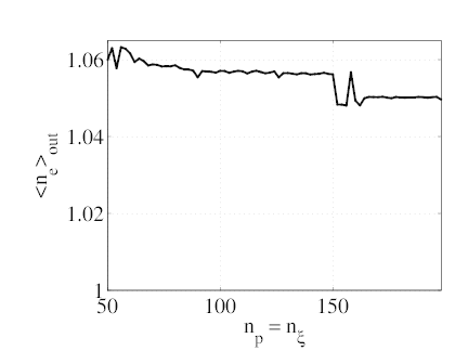
pmax = 10. The computed electron density increases slightly then stabilizes during the relaxation
and reaches an output value neout with (
,
which is taken to be uniform (Fig 7.17). The maximum momentum grid point is set at
pmax = 10. The computed electron density increases slightly then stabilizes during the relaxation
and reaches an output value neout with ( ∕ne ≤ 6%). This difference is quite small
given that a EC diffusion coefficient of D0ECnew = 0.15 is rather large. The output
density does not rapidly converge to 1 when the grid size in increased (graph a) which
indicates that the primary reason for the density increase is not the precision of the
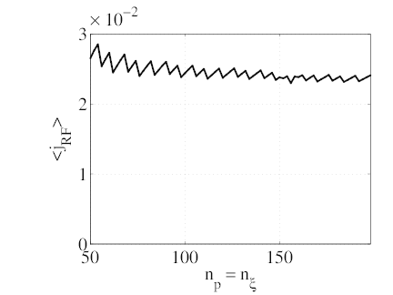
discretization scheme. The the flux-surface averaged driven current densiry (graph
b) converges towards a normalized asymptotic value j∞EC = 2.4 × 10⁻² (enevTe).
However, there are oscillations in the evolution of jEC with
∕ne ≤ 6%). This difference is quite small
given that a EC diffusion coefficient of D0ECnew = 0.15 is rather large. The output
density does not rapidly converge to 1 when the grid size in increased (graph a) which
indicates that the primary reason for the density increase is not the precision of the
discretization scheme. The the flux-surface averaged driven current densiry (graph
b) converges towards a normalized asymptotic value j∞EC = 2.4 × 10⁻² (enevTe).
However, there are oscillations in the evolution of jEC with  which account
for most of the disparity with j∞. These oscillations can be attributed to the sharp
Gaussian-like evolution of the diffusion coefficient in momentum space, with a characteristic
variation size that is smaller than a grid step. The gaussian shape of the spectrum being
somewhat smoother than the LH square spectrum, the variations in jEC are less
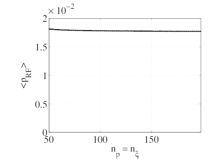
important than for the previous LH case. The calculation of the the flux-surface averaged
density of power absorbed (graph c) is however quite robust and does not depend much
on the grid size. It rapidly converges to a value p∞EC = 1.8 × 10⁻² (nemeνevTe2).
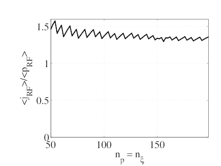
The evolution of the normalized figure of merit ηEC ≡ jEC∕pEC mostly follows the
variations of jEC (graph d). It converges to a value of η∞EC = 1.3 (e∕meνevTe). For a
100 × 100 grid, the mean error on jEC and ηEC is about 10%. It reduces to less than
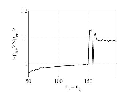
5% for a 200 × 200 grid. The ratio of the power absorbed from ECW to the power
lost on collisions expectedly tends to 1 as the grid size increases (graph e), until the
grid size reaches about 150 × 150, where it undergoes an unexplained jump to about
1.1.
which account
for most of the disparity with j∞. These oscillations can be attributed to the sharp
Gaussian-like evolution of the diffusion coefficient in momentum space, with a characteristic
variation size that is smaller than a grid step. The gaussian shape of the spectrum being
somewhat smoother than the LH square spectrum, the variations in jEC are less
important than for the previous LH case. The calculation of the the flux-surface averaged
density of power absorbed (graph c) is however quite robust and does not depend much
on the grid size. It rapidly converges to a value p∞EC = 1.8 × 10⁻² (nemeνevTe2).
The evolution of the normalized figure of merit ηEC ≡ jEC∕pEC mostly follows the
variations of jEC (graph d). It converges to a value of η∞EC = 1.3 (e∕meνevTe). For a
100 × 100 grid, the mean error on jEC and ηEC is about 10%. It reduces to less than
5% for a 200 × 200 grid. The ratio of the power absorbed from ECW to the power
lost on collisions expectedly tends to 1 as the grid size increases (graph e), until the
grid size reaches about 150 × 150, where it undergoes an unexplained jump to about
1.1.
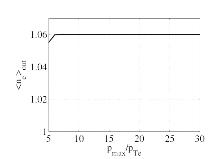
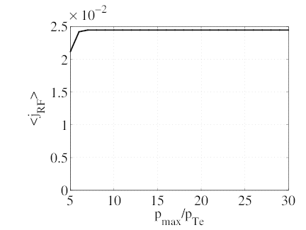
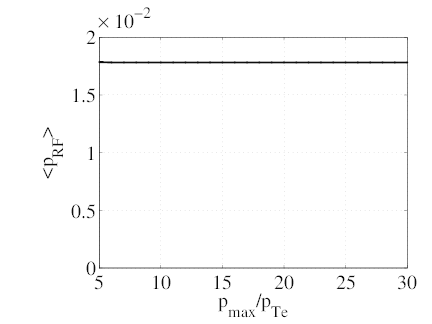
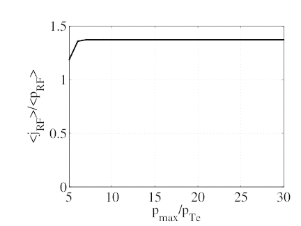
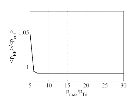
The requirements of ECCD calculations on the maximum momentum pmax are far more
easily satisfied than for LHCD. To illustrate this, we consider the same case (ρ = 0.1, θb = 0,
N∥ = 0.3, ΔN∥ = 0.02, y2 = 0.98, D0ECnew = 0.15) and fix nξ = 100. The maximum
momentum pmax and the momentum grid size np are varied proportionally so that the
momentum step size remains unchanged and the discretization effects are therefore removed.
The results are shown on Fig. 7.18. None of the relevant integral quantities (neout, jEC, pEC,
pEC∕pcol., ηEC) varies significantly for pmax∕pTe ≥ 7. For comparison, the maximum value
of p⊥ on the resonance curve is p⊥,maxres = 2.7pTe and the maximum value of p is
pmaxres = 6.4pTe.
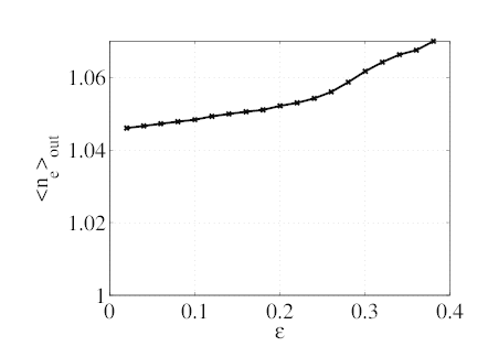
7.4.3 Electron trapping effects
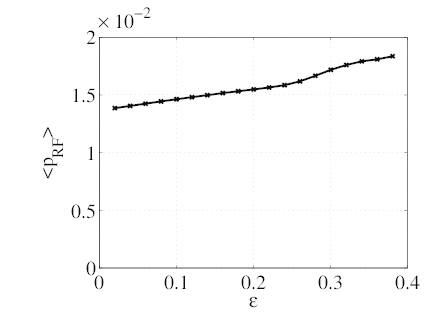
In the next set of calculation (Fig. 7.19), we keep the same ECCD parameters (θb = 0,
N∥ = 0.3, ΔN∥ = 0.02, y2 = 0.98, D0ECnew = 0.15) but vary the radial location of ECCD.
The density and temperature profiles are kept constant such that the only effect to
consider is the increasing number of trapped particles as ϵ = r∕Rp increases. The output
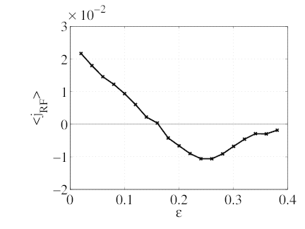
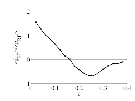
density increases slightly with ϵ (graph a) but remains acceptable. The density of driven
current steadily decreases and reverses signs for ϵ ≥ 0.16 (graph b). This evolution
indicates that the Ohkawa effect, which is due to ECW-induced trapping and drives a
counter-current, eventually compensates and even dominates the Fisch-Boozer effect. In fact,
the Ohkawa current density peaks at ϵ ≃ 0.25 and then  goes back to 0 as ϵ
further increases. The ohkawa effect is maximum where the EC resonance curve in
momentum space is tangent to the trapped passing boundary, so that wave-induced
trapping is maximum. For larger ϵ - or wider trapping region - most of the EC power is
transferred directly to trapped electrons, which do not drive current. This explains why
goes back to 0 as ϵ
further increases. The ohkawa effect is maximum where the EC resonance curve in
momentum space is tangent to the trapped passing boundary, so that wave-induced
trapping is maximum. For larger ϵ - or wider trapping region - most of the EC power is
transferred directly to trapped electrons, which do not drive current. This explains why
 → 0 as ϵ ≥ 0.25 increases. The density of power absorbed slowly increases with ϵ
(graph c). The increases is faster for ϵ ≥ 0.25, which can be expected since at these
location, increasing coupling with trapped particles occur. Indeed, because of the
fast bounce motion, this coupling is effectively distributed between trapped electrons
travelling in both directions. This distribution divides the effective magnitude of the
diffusion coefficient by two but also doubles the amount of resonant particles in the
trapped region. As a result, quasilinear effects on ECCD with trapped particles are
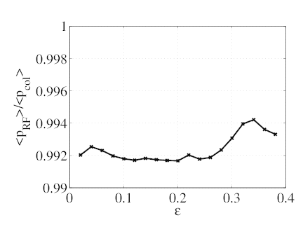
reduced, which explains the larger density of power absorbed. The evolution of the
normalized figure of merit is similar as that of
→ 0 as ϵ ≥ 0.25 increases. The density of power absorbed slowly increases with ϵ
(graph c). The increases is faster for ϵ ≥ 0.25, which can be expected since at these
location, increasing coupling with trapped particles occur. Indeed, because of the
fast bounce motion, this coupling is effectively distributed between trapped electrons
travelling in both directions. This distribution divides the effective magnitude of the
diffusion coefficient by two but also doubles the amount of resonant particles in the
trapped region. As a result, quasilinear effects on ECCD with trapped particles are
reduced, which explains the larger density of power absorbed. The evolution of the
normalized figure of merit is similar as that of  (graph d) and the ratio of he power
absorbed from ECW to the power lost on collisions is quite stable, and very close to
1.
(graph d) and the ratio of he power
absorbed from ECW to the power lost on collisions is quite stable, and very close to
1.
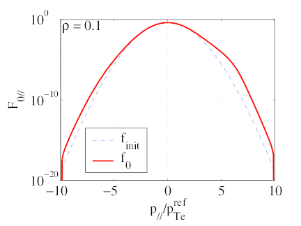
7.4.4 Momentum-space dynamics
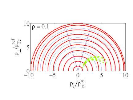
In order to illustrate the momentum-space dynamics of ECCD, the 2D distribution function is
plotted in the  space (Fig. 7.20). The case considered here is again our primary example
(ρ = 0.1, θb = 0, N∥ = 0.3, ΔN∥ = 0.02, y2 = 0.98, D0ECnew = 0.15). On graph a, the initial
Maxwellian (thin blue contours) and the steady-state ECCD distribution (thick red contours)
are displayed, as well as contour of the magnitude of the EC diffusion coefficient (green dashed
contours). The distortion of the distribution from a Maxwellian in the vicinity of the resonant
region is clearly visible. Collisions are trying to restore the Maxwellian and induce
momentum-space fluxes that affect the entire momentum space. By integrating over p⊥, we
obtain the parallel distribution
space (Fig. 7.20). The case considered here is again our primary example
(ρ = 0.1, θb = 0, N∥ = 0.3, ΔN∥ = 0.02, y2 = 0.98, D0ECnew = 0.15). On graph a, the initial
Maxwellian (thin blue contours) and the steady-state ECCD distribution (thick red contours)
are displayed, as well as contour of the magnitude of the EC diffusion coefficient (green dashed
contours). The distortion of the distribution from a Maxwellian in the vicinity of the resonant
region is clearly visible. Collisions are trying to restore the Maxwellian and induce
momentum-space fluxes that affect the entire momentum space. By integrating over p⊥, we
obtain the parallel distribution
 | (7.11) |
shown on graph b. In the non-relativistic limit, the integration of  F∥
F∥ over p∥ gives
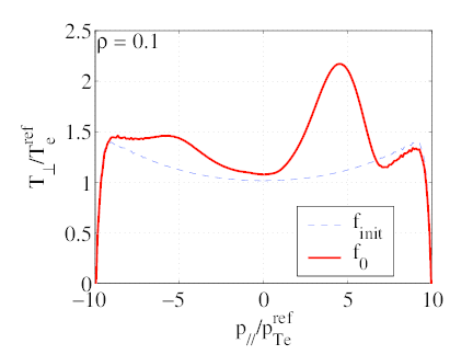
the driven current density. The Fisch-Boozer effect, resulting in an accumulation of particles
with large, positive p∥, appears clearly. This effect - understood as an asymmetric resistivity due
to EC heating - is also illustrated on graph c, where the perpendicular temperature is plotted as
a function of p∥; the difference in temperature, due to asymmetric EC heating, induces
the asymmetric resistivity and driven current. Note that EC induced diffusion in
momentum space is mostly in the perpendicular direction, and therefore does not directly
drive any current. It is always the collisional response to this diffusion which drives a
current.
over p∥ gives
the driven current density. The Fisch-Boozer effect, resulting in an accumulation of particles
with large, positive p∥, appears clearly. This effect - understood as an asymmetric resistivity due
to EC heating - is also illustrated on graph c, where the perpendicular temperature is plotted as
a function of p∥; the difference in temperature, due to asymmetric EC heating, induces
the asymmetric resistivity and driven current. Note that EC induced diffusion in
momentum space is mostly in the perpendicular direction, and therefore does not directly
drive any current. It is always the collisional response to this diffusion which drives a
current.
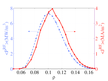
7.4.5 Coupling to propagation models
The code can be coupled to ray-tracing calculations. Iterations on the 3D ECCD
calculations ensure that the power absorbed from the EC wave is consistent with
the power travelling in the EC beam. Such calculations are very fast, thanks to the
fully-implicit 3D algorithm. To illustrate this, we consider a simplified ECCD scenario with
X-mode polarization, N∥ = 0.3, fEC = 110 MHz, P0EC = 1.0 MW and Gaussian
spectrum width ΔN∥ = 0.02. The EC beam propagates from the low field side on the
outboard midplane (θb = 0). The evolution of N∥ due to toroidicity is neglected, and the
cold plasma model is used to solve the dispersion relation. The DKE calculations
are performed on a nψ × np × nξ = 26 × 100 × 100 grid, and consistency between
travelling and absorbed power is reached after 4 iterations. The resultant current
density and absorbed power density profiles are shown on Fig. 7.21. The current profile
appears to be shifted slightly to the right compared to te power profile. This shift
results from the fact that at ρ ≥ 0.1, resonant electrons are further in the tail of the
distribution - meaning that they are less collisional - than at ρ ≤ 0.1, and therefore
the local efficiency is higher for ρ ≥ 0.1. The location ρ = 0.1 corresponds to the
peak in the absorbed power profile, which justifies taking this value for the previous
simulations.
7.4.6 Conclusion
To sum up, we have shown that the DKE code accurately describes and calculates ECCD. It
runs robustly in the free conservative mode. Grid parametric requirements are somewhat less
restrictive than for LHCD, because the EC diffusion coefficient variations are somewhat
smoother. It accounts correctly for trapped electron effects, such as the Ohkawa current. It can
be used to simulate actual ECCD scenarios, including coupling and consistency with ray-tracing
calculations.