Appendix F
Alternative discrete cross-derivatives coefficients
In Sec. 5.4.1, the discretization scheme is chosen so that cross-derivative terms
 l+1∕2,i+1∕2,j+1∕2 are all identical and defined at the center of each cell. Consequently,
cross-derivatives are determined in a completely symmetric way with respect to neighboring
points, which has be proven to be an efficient procedure for most simulation cases [?]. However,
the downside of this approach is that internal boundary conditions are no longer satisfied for
cross terms, and must be enforced. This is not a satisfactory situation particularly when a large
quasilinear diffusion takes place close to these locations of the phase space, in particular at
ξ0 = ±1.
l+1∕2,i+1∕2,j+1∕2 are all identical and defined at the center of each cell. Consequently,
cross-derivatives are determined in a completely symmetric way with respect to neighboring
points, which has be proven to be an efficient procedure for most simulation cases [?]. However,
the downside of this approach is that internal boundary conditions are no longer satisfied for
cross terms, and must be enforced. This is not a satisfactory situation particularly when a large
quasilinear diffusion takes place close to these locations of the phase space, in particular at
ξ0 = ±1.
Alternative discretization schemes may be considered in order to avoid this problem and
keep the treatment of internal boundaries in a uniform way for all derivatives. In this case,
Dpξ and Dξp
 are not separated from the derivatives of the distribution function as
done in Sec. 5.4.1, so that both
are not separated from the derivatives of the distribution function as
done in Sec. 5.4.1, so that both 
 and
and 
 must
directly discretized on the flux grid, according to the general rules. Coefficients are
therefore
must
directly discretized on the flux grid, according to the general rules. Coefficients are
therefore
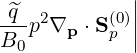
![^q ||(k+1) ^q m∑=8
---p2∇p ⋅S(p0)|| = --l+1∕2-- T[m]
B0 l+1∕2,i+1∕2,j+1∕2 B0,l+1∕2 m=1](NoticeDKE5492x.png) | (F.1) |
with
![(0)||(k+1)
- p2i+1D (p0p),l+1∕2,i+1,j+1∕2 ∂f∂0p-|| + p2i+1F (p0,l)+1∕2,i+1,j+1∕2f (00,)l+(k1+∕12),i+1,j+1∕2
T[1] =---------------------------l+1∕2,i+1,j+1∕2------------------------------------
Δpi+1∕2](NoticeDKE5493x.png) | (F.2) |
![(0) ∂f(0)||(k+1) (0) (0)(k+1)
p2iD pp,l+1∕2,i,j+1∕2 -0∂p-|| - p2iFp,l+1∕2,i,j+1∕2f0,l+1∕2,i,j+1∕2
T[2] = ---------------------l+1∕2,i,j+1∕2------------------------------
Δpi+1∕2](NoticeDKE5494x.png) | (F.3) |
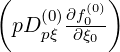
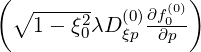
![∘ -----------
1 - ξ2 (0)||(k+1)
T [3] = +-------0,j+1∕2-pi+1D (0) ∂f0--||
Δpi+1∕2 pξ,l+1∕2,i+1,j+1∕2 ∂ξ0 |l+1∕2,i+1,j+1∕2](NoticeDKE5495x.png) | (F.4) |
![-----------
∘ 1 - ξ2 (0)||(k+1)
T [4] = --------0,j+1∕2pD (0) ∂f0--|
Δpi+1∕2 i pξ,l+1∕2,i,j+1∕2 ∂ξ0 ||
l+1∕2,i,j+1∕2](NoticeDKE5496x.png) | (F.5) |
![∘ -----2--- (0)|(k+1)
[7] ---pi+1∕2-----1---ξ0,j+1- l+1∕2,j+1 (0) ∂f-0-||
T = λl+1∕2,j+1∕2 Δ ξ0,j+1∕2 λ Dξp,l+1∕2,i+1∕2,j+1 ∂p ||
l+1 ∕2,i+1∕2,j+1](NoticeDKE5499x.png) | (F.8) |
![∘ ------- |
[8] pi+1∕2 1- ξ02,j l+1 ∕2,j (0) ∂f0(0)||(k+1)
T = - -l+1∕2,j+1∕2-Δ-ξ------λ D ξp,l+1∕2,i+1∕2,j-∂p--||
λ 0,j+1∕2 l+1∕2,i+1∕2,j](NoticeDKE5500x.png) | (F.9) |
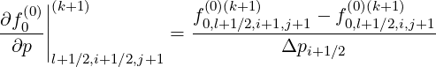
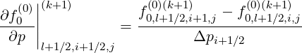
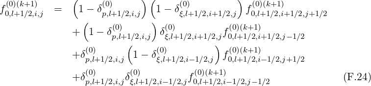
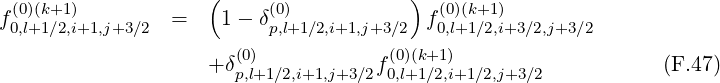
There are two methods for calculating derivatives of f0 that appear in the terms
T
that appear in the terms
T![[3]](NoticeDKE5502x.png) ,T
,T![[4]](NoticeDKE5503x.png) ,T
,T![[7]](NoticeDKE5504x.png) and T
and T![[8]](NoticeDKE5505x.png) . As shown in Fig.*** , it is possible to chose values of the distribution
function at all flux grid corners,
. As shown in Fig.*** , it is possible to chose values of the distribution
function at all flux grid corners,
 | (F.10) |
 | (F.11) |
 | (F.12) |
 | (F.13) |
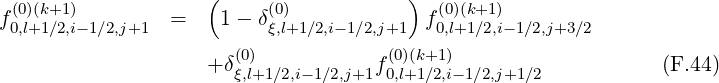
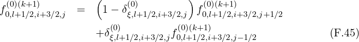
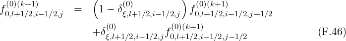
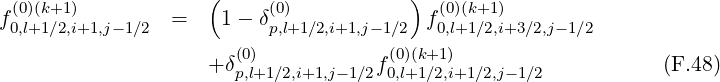
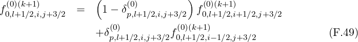
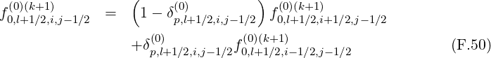
or to do it in an intermediate way,
 | (F.14) |
 | (F.15) |
 | (F.16) |
 | (F.17) |
involving flux grids only in the direction that is not considered by the derivative itself.
The advantage of this method is that the total number of interpolating coefficients δ
is reduced by a factor 2 as compared to the previous method, which represents a
significant numerical saving for the calculations. Nevertheless both methods are here
detailed.
It is important to notice that this new discretization scheme needs to evaluate now Dξp and
Dpξ
and
Dpξ at new grid points, i.e.
  ,
,  ,
, and
and  , while in the scheme discussed in Sec. 5.4.1, these coefficients were
determined only at the center of the cells
, while in the scheme discussed in Sec. 5.4.1, these coefficients were
determined only at the center of the cells  .
.
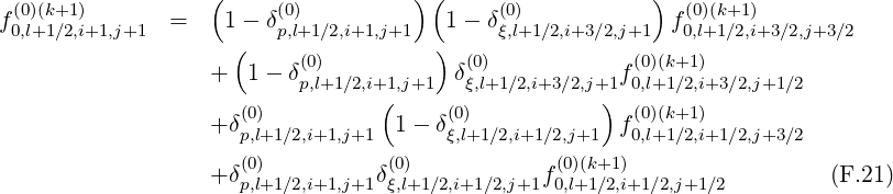
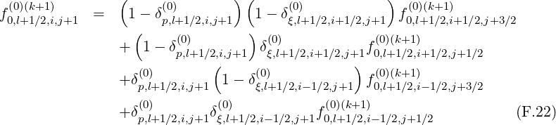
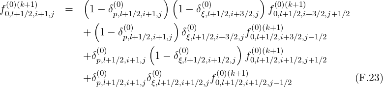
Full flux grid interpolation
Since the distribution function is defined on the half grid, while fluxes on the full grid, it is
necessary to interpolate, because in derivatives F.10-F.13, values of f0 are taken on the full
grid. In a general way, whatever the detailed value of the weighting factor δ
are taken on the full
grid. In a general way, whatever the detailed value of the weighting factor δ which will be
discussed in the Sec. 5.4.3, one may write for the terms proportional to Dpp
which will be
discussed in the Sec. 5.4.3, one may write for the terms proportional to Dpp , Fp
, Fp , Dξξ
, Dξξ and
Fξ
and
Fξ as in Sec. 5.4.1
For terms involving Dpξ and Dξp
 ,two steps interpolation must be carried out,
while and which leads to the result
By performing the appropriate index number transformations  and
and  other interpolations are
Gathering all terms, corresponding matrix coefficients for the zero order Fokker-Planck
equation may be expressed as
|  l+1∕2,i+1∕2,j+1∕2(k+1) l+1∕2,i+1∕2,j+1∕2(k+1) | |
|
| =  ∑
i′=i-1i′=i+1 ∑
j′=j-1j′=j+1M
p,l+1∕2,i′+1∕2,j′+1∕2 ∑
i′=i-1i′=i+1 ∑
j′=j-1j′=j+1M
p,l+1∕2,i′+1∕2,j′+1∕2 f
0,l+1∕2,i′+1∕2,j′+1∕2 f
0,l+1∕2,i′+1∕2,j′+1∕2 (k+1) (k+1) | (F.25) |
where
Terms proportional to Dξξ , Fξ
, Fξ and Dpp
 , Fp
, Fp are all gathered in matrix Mp
![[1]](NoticeDKE5548x.png) and
may be easily obtained from Mp
and
may be easily obtained from Mp given in Sec. 5.4.1 by taking Dpξ
 = Dξp
= Dξp = 0. The other
terms proportional to Dpξ
= 0. The other
terms proportional to Dpξ and Dξp
 are
are
Considerable simplifications occur for uniform momentum and pitch-angle grids. In that
case, δξ = δp
= δp = 1∕2, while Δp and Δξ0 are constant,
Half flux grid interpolation
In this case, a single interpolation step is necessary,
and
Matrix coefficients related to cross-derivatives are then
![--(0)[u]
M p,i+1∕2,j+1∕2 = 0](NoticeDKE5586x.png) | (F.55) |
and in the special case of uniform momentum and pitch-angle grids
![M-(0)[2u] = 0
p,i+1∕2,j+1∕2](NoticeDKE5595x.png) | (F.64) |
As expected, both methods merge for uniform momentum and pitch-angle grids, and matrix
coefficients for cross-derivatives are similar.
![⌊ ( ) (0)||(k+1)
| D(ξ0ξ),l+1∕2,i+1∕2,j+1 1 - ξ20,j+1 λl+1∕2,j+1 ∂f∂ξ00-||
T [5] = - --pi+1∕2---|| ------------------------------------------l+1∕2,i+1∕2,j+1-
λl+1∕2,j+1∕2 |⌈ .pi+1∕2Δ ξ0,j+1∕2
∘ ---------
p 1- ξ2 λl+1∕2,j+1F (0) f(0)(k+1) ⌋
+ -i+1∕2------0,j+1-----------ξ,l+1-∕2,i+1∕2,j+1-0,l+1∕2,i+1∕2,j+1⌉ (F.6)
Δ ξ0,j+1∕2](NoticeDKE5497x.png)
![⌊ ( ) (0)||(k+1)
| D (0ξξ),l+1∕2,i+1∕2,j 1 - ξ20,j λl+1∕2,j ∂f∂0ξ0-||
T [6] = ---pi+1∕2---|| ------------------------------------l+1∕2,i+1∕2,j-
λl+1∕2,j+1∕2|⌈ pi+1∕2Δ ξ0,j+1∕2
∘ -------
p 1- ξ2 λl+1∕2,jF (0) f(0)(k+1) ⌋
+ -i+1∕2------0,j--------ξ,l+1∕2,i+1∕2,j-0,l+1∕2,i+1∕2,j⌉ (F.7)
Δ ξ0,j+1∕2](NoticeDKE5498x.png)


![--- --- ---
M (p0,)l+1∕2,i′+1 ∕2,j′+1∕2 = M (0p,)l+[11]∕2,i′+1∕2,j′+1∕2 + M (0p,)l+[21]∕2,i′+1∕2,j′+1∕2](NoticeDKE5542x.png)
![∘1---ξ2------
---(0)[2] --------0,j+1∕2-- (0)
M p,l+1 ∕2,i+3∕2,j+3∕2 = + Δpi+1 ∕2Δ ξ0,j+1∕2pi+1D pξ,l+1∕2,i+1,j+1∕2
( (0) )( (0) )
× 1 - δp,l+1∕2,i+1,j+1 1- δξ,l+1∕2,i+3∕2,j+1
∘ ---------
pi+1∕2 1 - ξ20,j+1 l+1 ∕2,j+1 (0)
+ λl+1∕2,j+1∕2Δ-ξ-----Δp------λ D ξp,l+1∕2,i+1 ∕2,j+1
( 0,j+1∕2)( i+1∕2 )
× 1 - δ(0) 1- δ(0) (F.26)
p,l+1∕2,i+1,j+1 ξ,l+1∕2,i+3∕2,j+1](NoticeDKE5554x.png)
![-----------
∘ 1- ξ2
M--(0)[2] = + --------0,j+1∕2--p D(0)
p,l+1 ∕2,i+1∕2,j+3∕2 Δpi+1 ∕2Δ ξ0,j+1∕2 i+1 pξ,l+1∕2,i+1,j+1∕2
(0) ( (0) )
× δp,l+1∕2,i+1,j+1 1 - δξ,l+1∕2,i+1∕2,j+1
∘ ----2------
1- ξ0,j+1∕2 (0)
- Δp-----Δ-ξ------piDpξ,l+1∕2,i,j+1∕2
( i+1 ∕2 0,j+1∕2)( )
× 1 - δ(0) 1- δ(0)
p,l+1∕2,i,j∘+1-------ξ,l+1∕2,i+1∕2,j+1
p 1 - ξ20,j+1
+ ----i+1∕2-------------------λl+1 ∕2,j+1D (ξ0p),l+1∕2,i+1 ∕2,j+1
λl+1∕2,j+1∕2Δ ξ(0,j+1∕2Δpi+1 ∕2 )
× δ(0) 1 - δ(0)
p,l+1∕2,i+1,j+1∘ ----ξ,l+1∕2,i+1∕2,j+1
1 - ξ2
- ---pi+1∕2------------0,j+1---λl+1 ∕2,j+1D (0)
λl+1∕2,j+1∕2Δ ξ0,j+1∕2Δpi+1 ∕2 ξp,l+1∕2,i+1 ∕2,j+1
( (0) )( (0) )
× 1 - δp,l+1∕2,i,j+1 1- δξ,l+1∕2,i+1∕2,j+1 (F.27)](NoticeDKE5555x.png)
![∘ -----------
--- 1- ξ2
M--(0)[2] = - --------0,j+1∕2--p D(0)
p,l+1 ∕2,i-1∕2,j+3∕2 Δpi+1 ∕2Δ ξ0,j+1∕2 i pξ,l+1∕2,i,j+1∕2
(0) ( (0) )
× δp,l+1∕2,i,j+1 1 - δξ,l+1 ∕2,i-1∕2,j+1
∘ -----2---
---pi+1∕2-------1---ξ0,j+1--- l+1 ∕2,j+1 (0)
- λl+1∕2,j+1∕2Δ ξ Δp λ D ξp,l+1∕2,i+1 ∕2,j+1
( 0,j+1∕2 i+1∕2 )
× δ(p0),l+1∕2,i,j+1 1 - δ(0ξ),l+1 ∕2,i-1∕2,j+1 (F.28)](NoticeDKE5556x.png)
![∘1---ξ2------
---(0)[2] --------0,j+1∕2-- (0)
M p,l+1 ∕2,i+3∕2,j+1∕2 = + Δpi+1 ∕2Δ ξ0,j+1∕2pi+1D pξ,l+1∕2,i+1,j+1∕2
( (0) ) (0)
× 1 - δp,l+1∕2,i+1,j+1 δξ,l+1∕2,i+3∕2,j+1
∘ -----------
1- ξ20,j+1∕2 (0)
- Δp-----Δ-ξ------pi+1D pξ,l+1∕2,i+1,j+1∕2
( i+1 ∕2 0,j+1∕2)( )
× 1 - δ(0) 1- δ(0)
p,l+1∕2,i+1∘,j-------ξ,l+1∕2,i+3∕2,j
p 1 - ξ20,j+1
+ ----i+1∕2-------------------λl+1 ∕2,j+1D (ξ0p),l+1∕2,i+1 ∕2,j+1
λl+1∕2,j+1∕2Δ ξ0,j+1∕2Δpi+1 ∕2
( (0) ) (0)
× 1 - δp,l+1∕2,i+1,j+1-δξ,l+1∕2,i+3∕2,j+1
∘ 2
- ---pi+1∕2--------1---ξ0,j----λl+1 ∕2,jD (0)
λl+1∕2,j+1∕2Δ ξ0,j+1∕2Δpi+1 ∕2 ξp,l+1∕2,i+1∕2,j
( (0) )( (0) )
× 1 - δp,l+1∕2,i+1,j 1- δξ,l+1∕2,i+3∕2,j (F.29)](NoticeDKE5557x.png)
![∘1----ξ2-----
--(0)[2] --------0,j+1∕2-- (0)
M p,i+1∕2,j+1∕2 = + Δpi+1∕2Δ ξ0,j+1∕2 pi+1D pξ,l+1∕2,i+1,j+1∕2
(0) (0)
× δp,l+1∕2,i+1,j+1δξ,l+1∕2,i+1∕2,j+1
∘ -----2-----
---1---ξ0,j+1∕2-- (0)
- Δpi+1∕2Δ ξ0,j+1∕2 pi+1D pξ,l+1∕2,i+1,j+1∕2
( )
× δp(0,)l+1∕2,i+1,j 1- δ(ξ0,)l+1∕2,i+1∕2,j
∘ -----------
1 - ξ20,j+1∕2
- ----------------piD (p0)ξ,l+1∕2,i,j+1∕2
Δ(pi+1∕2Δ ξ0,j+1∕2)
× 1 - δ(0) δ(0)
∘ ---p,l+1-∕2,i,j+1 ξ,l+1∕2,i+1∕2,j+1
1 - ξ2
+ --------0,j+1∕2--piD (0)
Δpi+1∕2Δ ξ0,j+1∕2 pξ,l+1∕2,i,j+1∕2
( (0) ) ( (0) )
× 1 - δp,l+1 ∕2,i,j 1 - δξ,l+1 ∕2,i+1∕2,j
∘ -----2---
--pi+1∕2-------1---ξ0,j+1--- l+1∕2,j+1 (0)
+ λl+1∕2,j+1∕2 Δξ0,j+1∕2Δpi+1∕2λ D ξp,l+1 ∕2,i+1∕2,j+1
(0) (0)
× δp,l+1∕2,i+1,j+1δξ,l+1∕2,i+1∕2,j+1
∘ ---------
pi+1∕2 1 - ξ20,j+1 l+1∕2,j+1 (0)
- λl+1∕2,j+1∕2-Δξ------Δp-----λ D ξp,l+1 ∕2,i+1∕2,j+1
( 0,j+)1∕2 i+1∕2
× 1 - δ(0p,)l+1 ∕2,i,j+1 δ(ξ0,l)+1∕2,i+1∕2,j+1
∘ -------
p 1 - ξ20,j
- ---i+1∕2------------------λl+1∕2,jD (ξ0)p,l+1∕2,i+1∕2,j
λl+1∕2,j+1∕2 Δ(ξ0,j+1∕2Δpi+1∕2 )
× δ(0) 1- δ(0)
p,l+1∕2,i+1,j ∘ ξ,l+1∕2,i+1∕2,j
1 - ξ2
+ --pi+1∕2-------------0,j---λl+1∕2,jD (0)
λl+1∕2,j+1∕2 Δξ0,j+1∕2Δpi+1∕2 ξp,l+1∕2,i+1∕2,j
( (0) ) ( (0) )
× 1 - δp,l+1 ∕2,i,j 1 - δξ,l+1 ∕2,i+1∕2,j (F.30)](NoticeDKE5558x.png)
![∘ ----2------
---(0)[2] 1- ξ0,j+1∕2 (0)
M p,l+1 ∕2,i-1∕2,j+1∕2 = - Δp-----Δ-ξ------piDpξ,l+1∕2,i,j+1∕2
i+1 ∕2 0,j+1∕2
× δ(p0),l+1∕2,i,j+1 δ(0ξ,)l+1∕2,i-1∕2,j+1
∘ -----------
1- ξ20,j+1∕2 (0)
+ ----------------piDpξ,l+1∕2,i,j+1∕2
Δpi+1 ∕2Δ ξ(0,j+1∕2 )
× δ(0) 1 - δ(0)
p,l+1∕2,i,j ∘ ξ,l+1∕2,i-1∕2,j
1 - ξ2
- ---pi+1∕2------------0,j+1---λl+1 ∕2,j+1D (0)
λl+1∕2,j+1∕2Δ ξ0,j+1∕2Δpi+1 ∕2 ξp,l+1∕2,i+1 ∕2,j+1
(0) (0)
× δp,l+1∕2,i,j+1 δξ,l+1∘∕2,i-1∕2,j+1
1 - ξ2
+ ---pi+1∕2-------------0,j----λl+1 ∕2,jD (0)
λl+1∕2,j+1∕2Δ ξ0,j+1∕2Δpi+1 ∕2 ξp,l+1∕2,i+1∕2,j
(0) ( (0) )
× δp,l+1∕2,i,j 1 - δξ,l+1∕2,i-1∕2,j (F.31)](NoticeDKE5559x.png)
![∘ -----------
--(0)[2] 1- ξ20,j+1∕2
M p,l+1∕2,i+3∕2,j-1∕2 = - ----------------pi+1Dp(0ξ),l+1∕2,i+1,j+1∕2
Δ(pi+1 ∕2Δ ξ0,j+1∕2)
× 1- δ(0) δ(0)
p,l+1∕2,i+1∘,j -ξ,l+1∕2,i+3∕2,j
1- ξ2
- ---pi+1∕2-------------0,j----λl+1∕2,jD (0)
λl+1∕2,j+1∕2Δ ξ0,j+1∕2Δpi+1 ∕2 ξp,l+1∕2,i+1 ∕2,j
( (0) ) (0)
× 1- δp,l+1∕2,i+1,j δξ,l+1∕2,i+3∕2,j (F.32)](NoticeDKE5560x.png)
![∘ -----------
--- 1- ξ2
M-(0)[2] = - --------0,j+1∕2--p D (0)
p,l+1∕2,i+1∕2,j-1∕2 Δpi+1 ∕2Δ ξ0,j+1∕2 i+1 pξ,l+1∕2,i+1,j+1∕2
(0) (0)
× δp,l+1∕2,i+1,jδξ,l+1∕2,i+1∕2,j
∘ ----2------
----1--ξ0,j+1∕2-- (0)
+ Δpi+1 ∕2Δ ξ0,j+1∕2piDpξ,l+1∕2,i,j+1∕2
( (0) ) (0)
× 1- δp,l+1∕2,i,j δξ,l+1∕2,i+1∕2,j
∘ -------
pi+1∕2 1- ξ20,j (0)
- -l+1∕2,j+1∕2----------------λl+1∕2,jD ξp,l+1∕2,i+1 ∕2,j
λ Δ ξ0,j+1∕2Δpi+1 ∕2
× δ(0) δ(0)
p,l+1∕2,i+1,j ξ,l+1∘∕2,i+1∕2,j-
p 1- ξ20,j
+ -l+1i+∕12∕,j2+1∕2----------------λl+1∕2,jD (ξ0p),l+1∕2,i+1 ∕2,j
λ( Δ ξ0,)j+1∕2Δpi+1 ∕2
× 1- δ(0) δ(0) (F.33)
p,l+1∕2,i,j ξ,l+1∕2,i+1∕2,j](NoticeDKE5561x.png)
![∘1---ξ2------
--(0)[2] --------0,j+1∕2-- (0)
M p,l+1∕2,i-1∕2,j-1∕2 = + Δpi+1 ∕2Δ ξ0,j+1∕2piDpξ,l+1∕2,i,j+1∕2
(0) (0)
× δp,l+1∕2,i,jδξ,l+1∕2,i-1∕2,j
∘ ----2--
---pi+1∕2---------1--ξ0,j---- l+1∕2,j (0)
+ λl+1∕2,j+1∕2Δ ξ0,j+1∕2Δpi+1 ∕2λ D ξp,l+1∕2,i+1 ∕2,j
(0) (0)
× δp,l+1∕2,i,jδξ,l+1∕2,i-1∕2,j (F.34)](NoticeDKE5562x.png)
![∘ -----------
--- 1- ξ2
M-(0)[2u] = + ------0,j+1∕2p D (0)
p,l+1∕2,i+3∕2,j+3 ∕2 4Δp Δ ξ0 i+1 pξ,l+1∕2,i+1,j+1∕2
∘ -----2---
--pi+1∕2-----1---ξ0,j+1 l+1∕2,j+1 (0)
+ λl+1∕2,j+1∕2 4Δ ξ0Δp λ D ξp,l+1∕2,i+1∕2,j+1(F.35)](NoticeDKE5565x.png)
![∘1---ξ2------
--(0)[2u] ------0,j+1∕2- (0)
M p,l+1∕2,i+1∕2,j+3∕2 = + 4Δp Δ ξ0 pi+1D pξ,l+1∕2,i+1,j+1∕2
∘ ----2------
--1--ξ0,j+1∕2- (0)
- 4Δp Δ ξ0 piD pξ,l+1∕2,i,j+1∕2 (F.36)](NoticeDKE5566x.png)
![∘ -----------
--(0)[2u] 1- ξ2
M p,l+1∕2,i-1∕2,j+3 ∕2 = - ------0,j+1∕2piD (0)
4Δp Δ ξ0 ∘ ----pξ,l+1∕2,i,j+1∕2
1 - ξ2
- --pi+1∕2----------0,j+1λl+1∕2,j+1D (0) (F.37)
λl+1∕2,j+1∕2 4Δ ξ0Δp ξp,l+1∕2,i+1∕2,j+1](NoticeDKE5567x.png)
![∘ ---------
--(0)[2u] pi+1∕2 1 - ξ20,j+1 l+1∕2,j+1 (0)
M p,l+1∕2,i+3∕2,j+1 ∕2 = + -l+1∕2,j+1∕2--4Δ-ξ-Δp--λ D ξp,l+1∕2,i+1∕2,j+1
λ ∘ ----0--
p 1 - ξ20,j
- -l+1i∕+21,j∕2+1∕2---------λl+1∕2,jD (0ξp),l+1∕2,i+1∕2,j (F.38)
λ 4Δ ξ0Δp](NoticeDKE5568x.png)
![--(0)[2u]
M p,i+1∕2,j+1∕2 = 0](NoticeDKE5569x.png)
![∘ -----2---
--(0)[2u] --pi+1∕2-----1---ξ0,j+1 l+1∕2,j+1 (0)
M p,l+1∕2,i-1∕2,j+1 ∕2 = - λl+1∕2,j+1∕2 4Δ ξ0Δp λ D ξp,l+1∕2,i+1∕2,j+1
∘ -----2-
--pi+1∕2-----1---ξ0,j l+1∕2,j (0)
+ λl+1∕2,j+1∕2 4Δ ξ0Δp λ D ξp,l+1∕2,i+1∕2,j (F.39)](NoticeDKE5570x.png)
![∘ -----------
--(0)[2u] 1- ξ2
M p,l+1∕2,i+3∕2,j-1∕2 = - ------0,j+1∕2pi+1D (0)
4Δp Δ ξ0∘ -----pξ,l+1∕2,i+1,j+1∕2
1- ξ2
- --pi+1∕2---------0,jλl+1∕2,jD (0) (F.40)
λl+1∕2,j+1∕2 4Δ ξ0Δp ξp,l+1∕2,i+1∕2,j](NoticeDKE5571x.png)
![∘ -----------
--- 1- ξ2
M-(0)[2u] = - ------0,j+1∕2p D (0)
p,l+1∕2,i+1∕2,j-1∕2 4Δp Δ ξ0 i+1 pξ,l+1∕2,i+1,j+1∕2
∘ ----2------
--1--ξ0,j+1∕2- (0)
+ 4Δp Δ ξ0 piD pξ,l+1∕2,i,j+1∕2 (F.41)](NoticeDKE5572x.png)
![∘ -----------
--(0)[2u] 1- ξ20,j+1∕2
M p,l+1∕2,i-1∕2,j-1∕2 = + ------------piD (0pξ),l+1∕2,i,j+1∕2
4Δp Δ ξ0∘ -------
1- ξ2
+ --pi+1∕2---------0,jλl+1∕2,jD (0) (F.42)
λl+1∕2,j+1∕2 4Δ ξ0Δp ξp,l+1∕2,i+1∕2,j](NoticeDKE5573x.png)

![∘ -----------
--(0)[u] 1- ξ02,j+1 ∕2
M p,l+1∕2,i+3∕2,j+3∕2 = +------------------------pi+1D(p0ξ),l+1∕2,i+1,j+1∕2
Δp(i+1 ∕2(Δξ0,j+1 + Δ ξ)0,j)
× 1- δ(0)
p,l+1∕2,i+1,j+3∘∕2--------
1- ξ2
+---pi+1∕2---------------0,j+1------λl+1∕2,j+1D (0)
λl+1∕2,j+1∕2Δ ξ0,j+1∕2(Δpi+1 + Δpi) ξp,l+1 ∕2,i+1∕2,j+1
( (0) )
× 1- δξ,l+1∕2,i+3∕2,j+1 (F.51)](NoticeDKE5582x.png)
![∘ -----------
--- 1- ξ2
M--(0)[u] = ------------0,j+1∕2------p D(0)
p,l+1∕2,i+1∕2,j+3∕2 Δpi+1 ∕2(Δξ0,j+1 + Δ ξ0,j) i+1 pξ,l+1∕2,i+1,j+1∕2
(0)
× δp,l+1 ∕2,i+1,j+3∕2
∘ ----2------
--------1--ξ0,j+1∕2------ (0)
- Δpi+1∕2(Δ ξ0,j+1 + Δξ0,j)piD pξ,l+1∕2,i,j+1∕2
( (0) )
× 1 - δp,l+1∕2,i,j+3∕2 (F.52)](NoticeDKE5583x.png)
![∘ -----------
--(0)[u] 1- ξ2
M p,l+1∕2,i-1∕2,j+3∕2 = -------------0,j+1-∕2------piD(0)
Δpi+1 ∕2(Δξ0,j+1 + Δ ξ0,j) pξ,l+1∕2,i,j+1∕2
(0)
×δp,l+1∕2,i,j+3∕2 ∘ ---------
1- ξ2
----pi+1∕2---------------0,j+1------λl+1∕2,j+1D (0)
λl+1∕2,j+1∕2Δ ξ0,j+1∕2(Δpi+1 + Δpi) ξp,l+1 ∕2,i+1∕2,j+1
( (0) )
× 1- δξ,l+1∕2,i-1∕2,j+1 (F.53)](NoticeDKE5584x.png)
![∘ -----2-
--(0)[u] ---pi+1∕2------------1---ξ0,j------ l+1∕2,j (0)
M p,l+1∕2,i+3∕2,j+1∕2 = -λl+1∕2,j+1∕2Δ ξ0,j+1∕2(Δpi+1 + Δpi)λ D ξp,l+1∕2,i+1∕2,j
( )
× 1- δ(ξ0,)l+1∕2,i+3∕2,j
∘ ---------
pi+1∕2 1- ξ02,j+1 (0)
+--l+1∕2,j+1∕2----------------------λl+1∕2,j+1D ξp,l+1 ∕2,i+1∕2,j+1
λ Δ ξ0,j+1∕2(Δpi+1 + Δpi)
×δ(0) (F.54)
ξ,l+1∕2,i+3∕2,j+1](NoticeDKE5585x.png)
![∘ -----2-
--(0)[u] --pi+1∕2-----------1---ξ0,j------- l+1∕2,j (0)
M p,l+1∕2,i-1∕2,j+1∕2 = λl+1∕2,j+1 ∕2 Δξ0,j+1∕2(Δpi+1 + Δpi )λ Dξp,l+1∕2,i+1 ∕2,j
( (0) )
× 1- δξ,l+1∕2,i-1∕2,j
∘ ---------
pi+1∕2 1- ξ02,j+1 l+1∕2,j+1 (0)
-λl+1∕2,j+1∕2Δ-ξ------(Δp----+-Δp-)λ D ξp,l+1 ∕2,i+1∕2,j+1
0,j+1∕2 i+1 i
×δ(ξ0,l)+1∕2,i-1∕2,j+1 (F.56)](NoticeDKE5587x.png)
![∘ -------
--- 1- ξ2
M--(0)[u] = - ---pi+1∕2----------------0,j-------λl+1∕2,jD(0)
p,l+1∕2,i+3∕2,j-1∕2 λl+1∕2,j+1∕2 Δ ξ0,j+1∕2 (Δpi+1 + Δpi ) ξp,l+1∕2,i+1∕2,j
(0)
× δξ,l+1 ∕2,i+3∕2,j-------
∘ 1- ξ2
- ------------0,j+1∕2-----p D (0)
Δpi+1∕2(Δ ξ0,j+1 + Δξ0,j) i+1 pξ,l+1 ∕2,i+1,j+1∕2
( (0) )
× 1 - δp,l+1∕2,i+1,j-1∕2 (F.57)](NoticeDKE5588x.png)
![∘1---ξ2------
--(0)[u] ------------0,j+1∕2------ (0)
M p,l+1∕2,i+1∕2,j-1∕2 = - Δpi+1 ∕2 (Δ ξ0,j+1 + Δ ξ0,j)pi+1D pξ,l+1∕2,i+1,j+1∕2
(0)
× δp,l+1∕2,i+1,j-1∕2
∘ ----2------
--------1--ξ0,j+1∕2------ (0)
+ Δpi+1 ∕2 (Δ ξ0,j+1 + Δ ξ0,j)piD pξ,l+1∕2,i,j+1 ∕2
( )
× 1- δ(p0,l)+1∕2,i,j-1∕2 (F.58)](NoticeDKE5589x.png)
![∘ -------
--- 1- ξ2
M-(0)[u] = ---pi+1∕2----------------0,j-------λl+1∕2,jD (0)
p,l+1∕2,i-1∕2,j-1∕2 λl+1∕2,j+1∕2Δ ξ0,j+1∕2(Δpi+1 + Δpi) ξp,l+1∕2,i+1∕2,j
(0)
× δξ,l+1∕2,i-1∕2,j------
∘ 1 - ξ2
+ ------------0,j+1∕2-----p D (0)
Δpi+1∕2(Δ ξ0,j+1 + Δ ξ0,j) i pξ,l+1∕2,i,j+1∕2
(0)
× δp,l+1∕2,i,j-1∕2 (F.59)](NoticeDKE5590x.png)
![∘1---ξ2------
--(0)[2u] ------0,j+1∕2- (0)
M p,l+1∕2,i+3∕2,j+3 ∕2 = + 4Δp Δ ξ0 pi+1D pξ,l+1∕2,i+1,j+1∕2
∘ -----2---
--pi+1∕2-----1---ξ0,j+1 l+1∕2,j+1 (0)
+ λl+1∕2,j+1∕2 4Δ ξ0Δp λ D ξp,l+1∕2,i+1∕2,j+1(F.60)](NoticeDKE5591x.png)
![∘ -----------
--(0)[2u] 1- ξ2
M p,l+1∕2,i+1 ∕2,j+3∕2 = ------0,j+1∕2pi+1D (0)
∘4Δp-Δ-ξ0----- pξ,l+1 ∕2,i+1,j+1∕2
1- ξ2
--------0,j+1∕2piD (0) (F.61)
4Δp Δξ0 pξ,l+1∕2,i,j+1∕2](NoticeDKE5592x.png)
![∘ -----------
--(0)[2u] 1- ξ20,j+1∕2 (0)
M p,l+1∕2,i-1∕2,j+3 ∕2 = - --4Δp-Δ-ξ---piD pξ,l+1∕2,i,j+1∕2
0 ∘ ---------
p 1 - ξ20,j+1
- -l+1i∕+21,j∕2+1∕2-----------λl+1∕2,j+1D (ξ0)p,l+1∕2,i+1∕2,j+1(F.62)
λ 4Δ ξ0Δp](NoticeDKE5593x.png)
![∘ -------
--- 1 - ξ2
M-(0)[2u] = - --pi+1∕2----------0,jλl+1∕2,jD (0)
p,l+1∕2,i+3∕2,j+1 ∕2 λl+1∕2,j+1∕2 4Δ ξ0Δp ξp,l+1∕2,i+1∕2,j
∘ -----2---
--pi+1∕2-----1---ξ0,j+1 l+1∕2,j+1 (0)
+ λl+1∕2,j+1∕2 4Δ ξ0Δp λ D ξp,l+1∕2,i+1∕2,j+1(F.63)](NoticeDKE5594x.png)
![∘ -------
--- 1- ξ2
M (p0,l)[+2u1]∕2,i-1∕2,j+1 ∕2 = --pi+1∕2---------0,jλl+1∕2,jD (0)
λl+1∕2,j+1 ∕2 4Δ∘ ξ0Δp----- ξp,l+1∕2,i+1∕2,j
1 - ξ2
- --pi+1∕2----------0,j+1λl+1∕2,j+1D (0) (F.65)
λl+1∕2,j+1∕2 4Δ ξ0Δp ξp,l+1∕2,i+1∕2,j+1](NoticeDKE5596x.png)
![∘ -------
--- 1- ξ2
M-(0)[2u] = - --pi+1∕2---------0,jλl+1∕2,jD (0)
p,l+1∕2,i+3∕2,j-1∕2 λl+1∕2,j+1∕2 4Δ ξ0Δp ξp,l+1∕2,i+1∕2,j
∘ ----2------
--1--ξ0,j+1∕2- (0)
- 4Δp Δ ξ0 pi+1D pξ,l+1∕2,i+1,j+1∕2 (F.66)](NoticeDKE5597x.png)
![∘ -----------
--(0)[2u] 1- ξ20,j+1∕2
M p,l+1∕2,i+1∕2,j-1∕2 = - ------------pi+1D (0p)ξ,l+1∕2,i+1,j+1∕2
∘ 4Δp-Δ-ξ0---
1- ξ2
+ ------0,j+1∕2piD (0) (F.67)
4Δp Δ ξ0 pξ,l+1∕2,i,j+1∕2](NoticeDKE5598x.png)
![∘ ----2--
--(0)[2u] --pi+1∕2-----1--ξ0,j- l+1∕2,j (0)
M p,l+1∕2,i- 1∕2,j- 1∕2 = λl+1∕2,j+1∕2 4Δ ξ0Δp λ D ξp,l+1∕2,i+1∕2,j
∘ ----2------
---1--ξ0,j+1∕2 (0)
+ 4Δp Δξ0 piDpξ,l+1∕2,i,j+1∕2 (F.68)](NoticeDKE5599x.png)