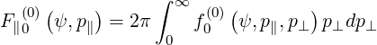
7.2 Runaway losses
Primary generation
The loss rate ΓR by primary runaway generation is also an important physical quantity that
can be determined by the code. It becomes significant when the Ohmic electric field is large. For
the benchmarking procedure, the Ohmic electric field is then set to E = 0.08, which corresponds
to a standard value for such studies. Usually, runaway losses become significant above E = 0.03.
All other parameters are kept constant as compared to the benchmarking procedure done for the
Ohmic conductivity in Sec. 7.1. In the tokamak parameter M-file “ptok_dke_1yp.m”, the
corresponding section for these simulations is named “CQL3D_RUNAWAY”, since it
corresponds to conditions that have been used for code comparison with the well know
CQL3D program ([?]). By definition, the code is no more conservative since runaway
electrons are leaving the domain of integration. Consequently, the particle losses must be
compensated in order to keep constant the total number of particle. Consequently, the same
Maxwellian solution is enforced at i = 1∕2 while the density is normalized at each iteration.
It has been cross-checked that the compensation of losses has no influence on the
final solution and therefore the runaway rate. Indeed, results normalized to the final
numerical electron density found by the code, or normalized at each time step are
similar.
In a first step, a local analysis is performed, without considering bounce averaging. Here,
only the Maxwellian electron-electron collision operator is considered, for allowing comparisons
with analytical solutions, as shown in 7.3
|
|
|
| Zeff | ΓR [DKE code] | ΓR [Kulsrud et al.] |
|
|
|
| 1 | 2.8487 × 10⁻⁴ | 3.177 × 10⁻⁴ |
|
|
|
| 2 | 1.5904 × 10⁻⁴ | 1.735 × 10⁻⁴ |
|
|
|
| 5 | 9.6565 × 10⁻⁵ | 1.047 × 10⁻⁴ |
|
|
|
| 10 | 8.1878 × 10⁻⁶ | 9.0 × 10⁻⁶ |
|
|
|
| |
Table 7.3: Runaway rate as function of the effective charge using the Maxwellian e-e
collision model
The agreement between numerical results obtained with the drift kinetic code and the code
written by Kulsrud and coauthors is reasonably good [?], a modest systematic difference of
-15% being observed for all Zeff values. For Zeff = 1, the agreement is slightly
better with the model of Kruskal-Bernstein [?], and the relative difference is now
positive and less than 7%. The role played by the numerical grid is marginal, less
than 1%. when np is varying from 88 to 125 or 165 while nξ0 is kept constant at
120.
The collision operator plays an important role in the value of ΓR. As shown in 7.4, using the
Belaiev-Budker operator with first order Legendre correction leads to twice more runaways than
expected by the model of Kruskal-Bernstein. The difference is even much larger with the model
of Connor and Hastie [?]. It must be emphasized that the expression of Møller for the
collision operator underestimate ΓR by 10% as compared to the high-velocity limit.
|
|
| Collision model | ΓR[Zeff = 1,E∕ED = 0.08] |
|
|
| Maxwellian (DKE) | 2.27 × 10⁻⁴ |
|
|
| High-velocity limit (DKE) | 2.10 × 10⁻⁴ |
|
|
| Belaiev-Budker (DKE) | 3.94 × 10⁻⁴ |
|
|
| Møller ultrarelativistic (DKE) | 1.99 × 10⁻⁴ |
|
|
| Kruskal-Bernstein | 2.67 × 10⁻⁴ |
|
|
| Connor-Hastie | 1.00 × 10⁻⁴ |
|
|
| |
Table 7.4: Runaway rate as function of the collision model. Calculations are performed
with bounce-averaging, which reduce ΓR by 21% as compared to data given in Table 7.3,
for similar plasma parameters.
A full 3 - D calculation has been performed with flat profiles at normalized radial
positions on the spatial flux grid ![[0.2,0.4,0.6,0.8]](NoticeDKE4213x.png) , giving the following radial positions
ρ =
, giving the following radial positions
ρ = ![[0.14142,0.31623, 0.5099,0.70711,0.90554]](NoticeDKE4214x.png) . In that case, the code calculates itself the
pitch-angle grid and the number of step is now nξ0 = 168, while np = 125.The runaway rate is
found to be independent of the method of calculations, and the Kruskal-Bernstein is well
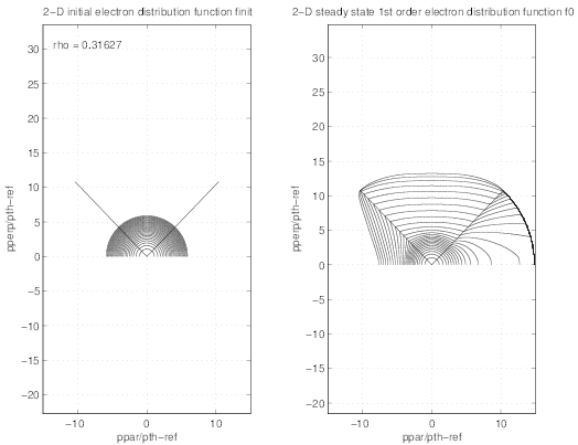
recovered when Zeff = 1 at all plasma radii. In Fig.7.2 , and example of a runaway distribution
at Bmin is given, for ρ = 0.31623. The trapped domain is large, and the region where the
electric field may accelerate fast electrons above the Dreicer limit is quite narrow in
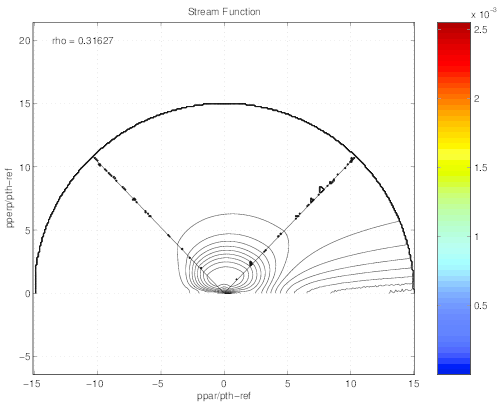
pitch-angle. The stream lines given in Fig.7.3 along with electrons are moving in the
momentum space show the clear boundary between close loops for regular electrons
that remain in the integration domain because of collisions, and the open loops, for
runaways that continuously accelerated by the Ohmic electric field up to the integration
domain.
. In that case, the code calculates itself the
pitch-angle grid and the number of step is now nξ0 = 168, while np = 125.The runaway rate is
found to be independent of the method of calculations, and the Kruskal-Bernstein is well
recovered when Zeff = 1 at all plasma radii. In Fig.7.2 , and example of a runaway distribution
at Bmin is given, for ρ = 0.31623. The trapped domain is large, and the region where the
electric field may accelerate fast electrons above the Dreicer limit is quite narrow in
pitch-angle. The stream lines given in Fig.7.3 along with electrons are moving in the
momentum space show the clear boundary between close loops for regular electrons
that remain in the integration domain because of collisions, and the open loops, for
runaways that continuously accelerated by the Ohmic electric field up to the integration
domain.
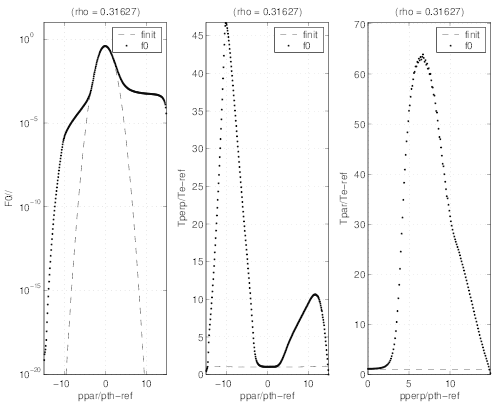
In Fig. 7.4, the parallel component of the electron distribution function
 | (7.4) |
the normalized perpendicular temperature T⊥ = T⊥
= T⊥ ∕Te† where
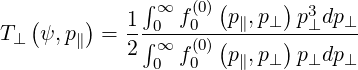 | (7.5) |
and the parallel one T∥ = T∥
= T∥ ∕Te† defined as
 | (7.6) |
are also given to illustrate the deformations of the electron distribution function with respect to
the Maxwellian shape.
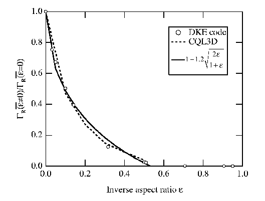
Bounce averaged calculations have be performed first locally. As shown in Fig. 7.5, it is
observed ΓR decreases with the inverse aspect ratio ϵ. The influence of toroidicity on Dreicer
generation, which is not predicted by the theory of Gurevitch [?], is in good agreement with
never published calculations using the CQL3D code. The explanation for such an effect is quite
complex, since it arises from the combination of the poloidal dependence of the electric field
value and the fact that trapped electrons do not contribute to the runaway generation process.
As shown in Sec. 3.6, the electric field on the low magnetic field side is lower than
the flux surface value, while it is larger on the high field side, by a ratio R0∕R for
circular concentric magnetic flux surfaces. So we could expect that these electrons are
more efficiently accelerated along bthe magnetic field line. But since they are close
to trapped/passing boundary, their probability to be trapped before reaching the
Dreicer limit is fairly high, and therefore, the density close to the Dreicer boundary
is likely significantly lowered. Consequently, the relative reduction of the runaway
rate
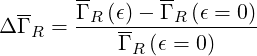 | (7.7) |
must be roughly given by a factor proportional to the effective fraction of trapped electron
 teff., since not only trapped but also barely trapped electron dynamics are concerned. A fit of
the numerical results confirms this coarse analysis, since
teff., since not only trapped but also barely trapped electron dynamics are concerned. A fit of
the numerical results confirms this coarse analysis, since
 | (7.8) |
for ϵ ≲ 0.53 and
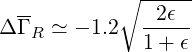
limϵ→0ΔΓR ≃ 1.7
≃ 1.7 ≃-1.16
teff..
This result is important, since it indicates that runaway generation is nearly cancelled when the
inverse aspect ratio is larger than ϵ ≃ 0.5. The trapped particles have therefore a beneficial effect
by preventing runaways, that may cause severe damages to machine walls in case of
disruptions.
≃-1.16
teff..
This result is important, since it indicates that runaway generation is nearly cancelled when the
inverse aspect ratio is larger than ϵ ≃ 0.5. The trapped particles have therefore a beneficial effect
by preventing runaways, that may cause severe damages to machine walls in case of
disruptions.
Similar results are obtained in 3 - D mode, whatever the normalization reference of the
electric field, at the plasma center, or at the local position. As expected, the runaway
rate ΓR is nearly independent of the sign of the electric field, and moreover, but also
of the method (analytical or numerical) for calculating the bounce integrals. The
relative accuracy which is less than 1% close to the plasma center, tends to decrease
down to 50% at the plasma edge, but since ΓR is very small the error has only a weak
influence.
Once more, this demonstrates that numerical calculations of the bounce integrals is very
accurate, even for finite inverse aspect ratio. The drop tolerance has been lowered in that
case to 10-4 for ensuring a stable convergence, leading to a modest increase of the
matrix sizes. However the rate of convergence is not affected, and the final result
is obtained usually after 11 - 13 iterations, even when several radial positions are
considered.
Secondary generation
The problem of secondary runaway generation is*****