5.8 Moments of the Distribution Function
5.8.1 Flux discretization for moment calculations
The calculation of momentum-space moments of the distribution function, such as the density of
power absorbed or the stream function, requires to calculate the bounce-averaged
momentum space fluxes Sp(0) associated with a distribution function. Considering a given
distribution function f (which could be f0
 ,
, 
 or g
or g ) and given momentum-space
diffusion Dp
) and given momentum-space
diffusion Dp
 and convection Fp
 coefficients, associated with a particular physical
mechanism
coefficients, associated with a particular physical
mechanism  (such as collisions, RF waves and DC electric field) and calculated in
chapter 4, these fluxes are given by (3.187) or equivalently (3.216) and their components
are
(such as collisions, RF waves and DC electric field) and calculated in
chapter 4, these fluxes are given by (3.187) or equivalently (3.216) and their components
are
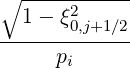
| Sp(0) | = -D
pp(0) + +  Dpξ(0) Dpξ(0) + Fp(0)f(0) + Fp(0)f(0) | (5.557)
|
| Sξ0(0) | = -D
ξp(0) + +  Dξξ(0) Dξξ(0) + Fξ(0)f(0) + Fξ(0)f(0) | (5.558) |
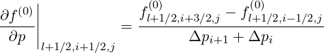
- First, both for power density (5.580) and stream function calculations (5.583), we need to
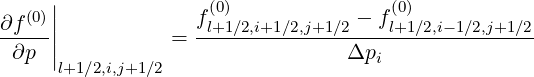
calculate the discretized flux Sp(0) at the flux grid point
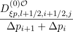
Sp,l+1∕2,i,j+1∕2 | = -D
pp,l+1∕2,i,j+1∕2(0) l+1∕2,i,j+1∕2 l+1∕2,i,j+1∕2 | (5.559)
|
| +  Dpξ,l+1∕2,i,j+1∕2(0) Dpξ,l+1∕2,i,j+1∕2(0) l+1∕2,i,j+1∕2 l+1∕2,i,j+1∕2 | |
|
| + Fp,l+1∕2,i,j+1∕2(0)f
l+1∕2,i,j+1∕2(0) | | |
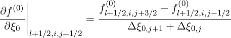
The first derivative is straightforward (5.58)
 | (5.560) |
while the second derivative, similar to (5.60)
 | (5.561) |
and the convective term both requires further interpolation (5.67)
fl+1∕2,i,j+3∕2 | = 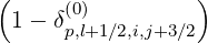 fl+1∕2,i+1∕2,j+3∕2 fl+1∕2,i+1∕2,j+3∕2 + δ
p,l+1∕2,i,j+3∕2 + δ
p,l+1∕2,i,j+3∕2 f
l+1∕2,i-1∕2,j+3∕2 f
l+1∕2,i-1∕2,j+3∕2 |
(5.562)
|
fl+1∕2,i,j+1∕2 | = 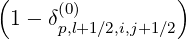 fl+1∕2,i+1∕2,j+1∕2 fl+1∕2,i+1∕2,j+1∕2 + δ
p,l+1∕2,i,j+3∕2 + δ
p,l+1∕2,i,j+3∕2 f
l+1∕2,i-1∕2,j+1∕2 f
l+1∕2,i-1∕2,j+1∕2 |
(5.563)
|
fl+1∕2,i,j-1∕2 | = 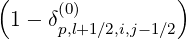 fl+1∕2,i+1∕2,j-1∕2 fl+1∕2,i+1∕2,j-1∕2 + δ
p,l+1∕2,i,j-1∕2 + δ
p,l+1∕2,i,j-1∕2 f
l+1∕2,i-1∕2,j-1∕2 f
l+1∕2,i-1∕2,j-1∕2 |
(5.564) |
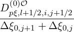
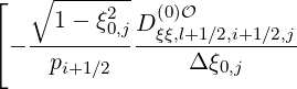
The expanded expression is then
Sp,l+1∕2,i,j+1∕2 | = 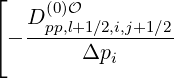 | |
|
| ![(0)O ( (0) ) ]
+F p,l+1∕2,i,j+1∕2 1 - δp,l+1∕2,i,j+1∕2](NoticeDKE3790x.png) fl+1∕2,i+1∕2,j+1∕2 fl+1∕2,i+1∕2,j+1∕2 | (5.565)
|
| + 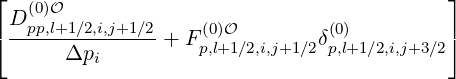 fl+1∕2,i-1∕2,j+1∕2 fl+1∕2,i-1∕2,j+1∕2 | |
|
| +    fl+1∕2,i+1∕2,j+3∕2 fl+1∕2,i+1∕2,j+3∕2 | |
|
| +   δp,l+1∕2,i,j+3∕2 δp,l+1∕2,i,j+3∕2 f
l+1∕2,i-1∕2,j+3∕2 f
l+1∕2,i-1∕2,j+3∕2 | |
|
| -   fl+1∕2,i+1∕2,j-1∕2 fl+1∕2,i+1∕2,j-1∕2 | |
|
| -  δp,l+1∕2,i,j-1∕2 δp,l+1∕2,i,j-1∕2 f
l+1∕2,i-1∕2,j-1∕2 f
l+1∕2,i-1∕2,j-1∕2 | | |
- For Stream function calculations (5.585), we also need to calculate the discretized flux
Sξ(0) at the flux grid point
Sξ,l+1∕2,i+1∕2,j | = -D
ξp,l+1∕2,i+1∕2,j(0) l+1∕2,i+1∕2,j l+1∕2,i+1∕2,j | (5.566)
|
| +  Dξξ,l+1∕2,i+1∕2,j(0) Dξξ,l+1∕2,i+1∕2,j(0) l+1∕2,i+1∕2,j l+1∕2,i+1∕2,j | |
|
| + Fξ,l+1∕2,i+1∕2,j(0)f
l+1∕2,i+1∕2,j(0) | | |
The first derivative is similar to (5.57)
 | (5.567) |
while the second is given by (5.61)
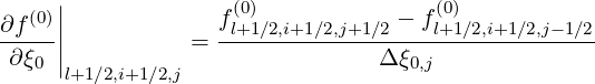 | (5.568) |
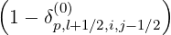
The first diffusion term and the convective term both requires further interpolation
(5.69)
fl+1∕2,i+3∕2,j | =  fl+1∕2,i+3∕2,j+1∕2 fl+1∕2,i+3∕2,j+1∕2 + δ
ξ,l+1∕2,i+3∕2,j + δ
ξ,l+1∕2,i+3∕2,j f
l+1∕2,i+3∕2,j-1∕2 f
l+1∕2,i+3∕2,j-1∕2 |
(5.569)
|
fl+1∕2,i+1∕2,j | =  fl+1∕2,i+1∕2,j+1∕2 fl+1∕2,i+1∕2,j+1∕2 + δ
ξ,l+1∕2,i+1∕2,j + δ
ξ,l+1∕2,i+1∕2,j f
l+1∕2,i+1∕2,j-1∕2 f
l+1∕2,i+1∕2,j-1∕2 |
(5.570)
|
fl+1∕2,i-1∕2,j | =  fl+1∕2,i-1∕2,j+1∕2 fl+1∕2,i-1∕2,j+1∕2 + δ
ξ,l+1∕2,i-1∕2,j + δ
ξ,l+1∕2,i-1∕2,j f
l+1∕2,i-1∕2,j-1∕2 f
l+1∕2,i-1∕2,j-1∕2 |
(5.571) |
The expanded expression is then
Sξ,l+1∕2,i+1∕2,j | =  | |
|
| ![(0)O ( (0) ) ]
+F ξ,l+1∕2,i+1∕2,j 1 - δξ,l+1∕2,i+1∕2,j](NoticeDKE3834x.png) fl+1∕2,i+1∕2,j+1∕2 fl+1∕2,i+1∕2,j+1∕2 | (5.572)
|
| +  | |
|
| ![(0)O (0) ]
+F ξ,l+1∕2,i+1∕2,jδξ,l+1 ∕2,i+1∕2,j](NoticeDKE3837x.png) fl+1∕2,i+1∕2,j-1∕2 fl+1∕2,i+1∕2,j-1∕2 | |
|
| -  fl+1∕2,i+3∕2,j+1∕2 fl+1∕2,i+3∕2,j+1∕2 | |
|
| - δξ,l+1∕2,i+3∕2,j δξ,l+1∕2,i+3∕2,j f
l+1∕2,i+3∕2,j-1∕2 f
l+1∕2,i+3∕2,j-1∕2 | |
|
| +   fl+1∕2,i-1∕2,j+1∕2 fl+1∕2,i-1∕2,j+1∕2 | |
|
| +  δξ,l+1∕2,i-1∕2,j δξ,l+1∕2,i-1∕2,j f
l+1∕2,i-1∕2,j-1∕2 f
l+1∕2,i-1∕2,j-1∕2 | | |
5.8.2 Numerical integrals for moment calculations
Density
From calculations in Sec.3.6, the flux surface averaged density  V,l+1∕2 at ψl+1∕2 may be
expressed as a sum of three terms
V,l+1∕2 at ψl+1∕2 may be
expressed as a sum of three terms

the first one corresponding to the zero order Fokker-Planck equation
 | (5.573) |
while the two others result from the solution of the electron drift kinetic equation
 | (5.574) |
and
 | (5.575) |
Current Density
In a similar way, the flux surface averaged parallel current  ϕ,l+1∕2 at ψl+1∕2 may be
expressed as a sum of three terms
ϕ,l+1∕2 at ψl+1∕2 may be
expressed as a sum of three terms
 | (5.576) |
where the zero order term is
|  ϕ,l+1∕20 = ϕ,l+1∕20 =   ∑
i=0np-1 ∑
j=0nξ0-1 ∑
i=0np-1 ∑
j=0nξ0-1 H H | |
|
| × ξ0,j+1∕2f0,l+1∕2,i+1∕2,j+1∕2(0)Δp
i+1∕2Δξ0,j+1∕2 | (5.577) |
The first order term arising from function g is
|  ϕ,l+1∕21 = ϕ,l+1∕21 =   ∑
i=0np-1 ∑
j=0nξ0-1 ∑
i=0np-1 ∑
j=0nξ0-1 H H | |
|
| × ξ0,j+1∕2gl+1∕2,i+1∕2,j+1∕2(0)Δp
i+1∕2Δξ0,j+1∕2 | (5.578) |
while the other one which results from  is more complex and
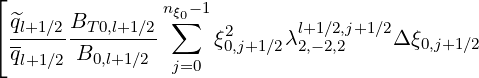
|  ϕ,l+1∕21 = ϕ,l+1∕21 =     ∑
i=0np-1 ∑
j=0nξ0-1 ∑
i=0np-1 ∑
j=0nξ0-1 λ2,-2,2l+1∕2,j+1∕2 λ2,-2,2l+1∕2,j+1∕2 | |
|
| × ξ0,j+1∕2 l+1∕2,i+1∕2,j+1∕2(0)Δp
i+1∕2Δξ0,j+1∕2. l+1∕2,i+1∕2,j+1∕2(0)Δp
i+1∕2Δξ0,j+1∕2. | (5.579) |
Power Density Associated with a Flux
The density of power absorbed by the plasma through a particular mechanism is the
sum

where the respective contributions are given by the equations (3.322) and (3.324-3.325) and
discretized as
 V,l+1∕20 V,l+1∕20 | =   ∑
i=1np
∑
j=0nξ0-1 ∑
i=1np
∑
j=0nξ0-1 λl+1∕2,j+1∕2S
p,l+1∕2,i,j+1∕2 λl+1∕2,j+1∕2S
p,l+1∕2,i,j+1∕2  ΔpiΔξ0,j+1∕2 ΔpiΔξ0,j+1∕2 |
(5.580)
|
 V,l+1∕21 V,l+1∕21 | =   ∑
i=1np
∑
j=0nξ0-1 ∑
i=1np
∑
j=0nξ0-1 λl+1∕2,j+1∕2S
p,l+1∕2,i,j+1∕2 λl+1∕2,j+1∕2S
p,l+1∕2,i,j+1∕2  ΔpiΔξ0,j+1∕2 ΔpiΔξ0,j+1∕2 |
(5.581)
|
 V,l+1∕21 V,l+1∕21 | =   ∑
i=1np
∑
j=0nξ0-1 ∑
i=1np
∑
j=0nξ0-1 λl+1∕2,j+1∕2 λl+1∕2,j+1∕2 p,l+1∕2,i,j+1∕2
  ΔpiΔξ0,j+1∕2 ΔpiΔξ0,j+1∕2 |
(5.582) |
The discretization of the momentum-space flux components Sp,l+1∕2,i,j+1∕2 and
and
 p,l+1∕2,i,j+1∕2
 is done in (5.565).
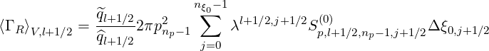
Stream Function for Momentum Space fluxes
The stream function gives the local direction of the momentum-space fluxes, and its gradient is
an indication of the flux intensity. Because it is a flux function, it is naturally defined on the
momentum-space flux grid. According to the three equivalent expressions for the
stream function (3.352-3.353), we have the following discretizations, for 1 ≤ i ≤ np and
1 ≤ j ≤ nξ - 1
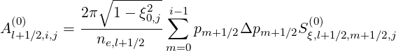
Al+1∕2,i,j | =  ∑
m=0j-1Δξ
0,m+1∕2Sp,l+1∕2,i,m+1∕2 ∑
m=0j-1Δξ
0,m+1∕2Sp,l+1∕2,i,m+1∕2 | (5.583)
|
Al+1∕2,i,j | =  ∑
m=jnξ-1Δξ
0,m+1∕2Sp,l+1∕2,i,m+1∕2 ∑
m=jnξ-1Δξ
0,m+1∕2Sp,l+1∕2,i,m+1∕2 | (5.584) |
and
 | (5.585) |
where the boundary conditions are
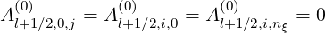 | (5.586) |
The discretization of the momentum-space flux components Sp,l+1∕2,i,j+1∕2 and
Sξ,l+1∕2,i+1∕2,j
and
Sξ,l+1∕2,i+1∕2,j is done in (5.565) and (5.572).
Ohmic electric field
As shown in Sec. 4.2, the flux surface averaged parallel Ohmic electrid field  ϕ
ϕ may be
expressed as a function of its local value E∥0
may be
expressed as a function of its local value E∥0 taken at the poloidal position where the
magnetic field B is minimum, and
taken at the poloidal position where the
magnetic field B is minimum, and
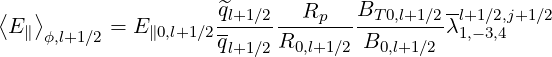 | (5.587) |
Exact and effective fractions of trapped electrons
The exact fraction of trapped electrons is given by relation,
|  t,l+1∕2 = t,l+1∕2 = 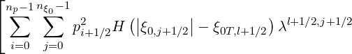 | |
|
| ×![( ) ]
^f(l+0)1∕2,i+1∕2,j+1∕2 + g(l0+)1∕2,i+1∕2,j+1∕2 Δpi+1∕2Δξ0,j+1∕2](NoticeDKE3914x.png) | |
|
| ×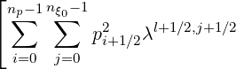 | |
|
| ×![( (0) ^(0) (0) ) ]
f0,l+1∕2,i+1∕2,j+1∕2 + fl+1∕2,i+1∕2,j+1∕2 + gl+1∕2,i+1∕2,j+1∕2 Δpi+1 ∕2Δ ξ0,j+1∕2](NoticeDKE3916x.png) -1 -1 | |
|
| | (5.588) |
according to calculations given in Sec. 3.6.
The effective fraction of trapped electrons, as deduced from the Lorentz model in Sec. 5.6.2
is
| t,l+1∕2eff. | =   × × | |
|
|  | |
|
|  | |
|
| ×![( || ||) ]
ξ0,j+1∕2IL ψl+1∕2,ξ0,j+1∕2 Δ ξ0,j+1∕2](NoticeDKE3921x.png) | (5.589) |
Runaway loss rate
As shown in Sec. 3.6, the runaway loss rate  V
V  is given
 | (5.590) |
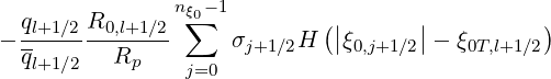
Magnetic ripple losses
In a similar way, the magnetic ripple loss rate ΓST 
 is given by
ΓST,l+1∕2 | = 2πp
ic2 ∑
j=0nξ0-1λl+1∕2,j+1∕2 Sp,l+1∕2,ic,j+1∕2 Sp,l+1∕2,ic,j+1∕2 Δξ
0,j+1∕2 Δξ
0,j+1∕2 | |
|
| + 4πλl+1∕2,jST
 ∑
i=0np-1p
i+1∕2H ∑
i=0np-1p
i+1∕2H Sξ0,l+1∕2,i+1∕2,jST Sξ0,l+1∕2,i+1∕2,jST Δp
i+1∕2 Δp
i+1∕2 |
(5.591) |
and the second formulation given in Sec.3.6 is
ΓST,l+1∕2 | = 2π ∑
i=0np-1 ∑
j=0nξ0-1 H H | |
|
| × νdST,l+1∕2,i+1∕2,j+1∕2f0,l+1∕2,i+1∕2,j+1∕2(0)Δξ
0,j+1∕2Δpi+1∕2 | (5.592) |
where ic is the index number that corresponds to the detrapping threshold by collisions,
and ξ0ST,l+1∕2 is the picth-angle boundary value between super-trapped and trapped
electrons.
Non-thermal bremsstrahlung
For the bremsstrahlung emission, it is necessary to calculate numericaly all coefficients of the
Legendre series. Since Legendre polynomials Pm strongly oscillate between -1 and +1,
as their order m increases, it is not possible to evaluate accurately integrals of the
type
 | (5.593) |
by standard integration techniques, like trapezoidal or Simpson rules. The only possibility is to
replace integral (5.593) by a discrete sum, namely a Gaussian quadrature,
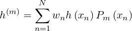 | (5.594) |
where weights wn and abscissas xn are determined independently. Here, the use of Legendre
polynomials lead to consider the fast ans accurate Gauss-Legendre algorithm as derived by G. B.
Ribicki in Ref. [?], where xn are N zeros of the Legendre polynomial of degree N, the weights
being given by the relation
![---------2--------
wn = 2 [ ′ ]2
(1 - xn) PN (xn)](NoticeDKE3938x.png) | (5.595) |
Very accurate determination of h may be obtained by this method, which requires a value
of N = 50.
may be obtained by this method, which requires a value
of N = 50.