
The 3 - D relativistic and bounce-averaged electron drift kinetic solver allows kinetic calculations of the bootstrap current for arbitrary tokamak magnetic configuration and in principle any type of electron velocity distribution function. Consequently, it offers for the first time the possibility to evaluate accurately potential synergistic effects due to external perturbations like application of RF waves. Indeed, so far, in all current drive simulations, the bootstrap current due to plasma pressure gradient is determined in the Maxwellian limit, while plasma may be locally far from the thermal regime during non inductive current drive. With this code, a self-consistent description of all current sources may be performed.
At this stage, this section is only given to demonstrate code performances in simple limits, like using the simplified Lorentz model, or for a Maxwellian plasma. Indeed, since there is no possibility to perform any benchmark in presence of RF current drive, this problem is not addressed here.
As shown in Sec.5.6.2, the Lorentz model applied to thermal plasma represents a unique opportunity for benchmarking the 3 - D drift kinetic code against simple analytical results. Here, comparisons are presented for a circular magnetic equilibrium, using numerical bounce integrals7. As for the electrical conductivity problem addressed in Sec.7.1, the minor radius is set to ap = 2.3899m and the major one is Rp = 2.39m so that the normalized radius ρ is very close to ϵ value from 0 to 1. Global parameters of the discharge are gathered in section “TEST_LORENTZ” of the tokamak parameter M-file “ptok_dke_1yp.m”. In order to simplify calculations, and identify clearly the pitch-angle dynamics that plays a major role in the bootstrap current calculation, all temperatures profiles are taken flat, and consequently the pressure profile arises only from density gradient. Its radial dependence is
|
| (7.14) |
where the central electron density is ne0 = 2 × 10+19m-3, and nea∕ne0 = 10-3. Electron temperature is taken low enough to neglect relativistic corrections, while Ts∕Te = 10-2, to simulate that ion background is fully cold. The dominant ion charge is taken Zs = 30, in agreement with basic assumptions of the Lorentz model.
In the simulation, the spatial ψ half-grid, on which the electron distribution function is
calculated, is highly non-uniform. Indeed, the effective spatial mesh size where bootstrap
current is determined has nψ - 1 = 14 points, but the distribution function f0 must be evaluated on 14 × 3 = 42 values of ψ for spatial gradients calculation by the
parabolic interpolation technique discussed in Sec.5.5.1 which requires 2 additional
neighboring points. Their distances to an effective point never exceed Δψ ≤ 0.01. The
fact that calculations may be easily performed with so close radial points is a good
indication of code capabilities for describing bootstrap current in presence of strong
pressure gradients. The pitch-angle grid is therefore also strongly non uniform, like
in Fig.7.23 for the Lower current drive problem, since trapped/passing boundaries
corresponding to all radial positions are exactly placed on the flux grid in momentum space.
Despite the number of ψ values is three times larger, the total number of pitch-angle
points for f0
must be evaluated on 14 × 3 = 42 values of ψ for spatial gradients calculation by the
parabolic interpolation technique discussed in Sec.5.5.1 which requires 2 additional
neighboring points. Their distances to an effective point never exceed Δψ ≤ 0.01. The
fact that calculations may be easily performed with so close radial points is a good
indication of code capabilities for describing bootstrap current in presence of strong
pressure gradients. The pitch-angle grid is therefore also strongly non uniform, like
in Fig.7.23 for the Lower current drive problem, since trapped/passing boundaries
corresponding to all radial positions are exactly placed on the flux grid in momentum space.
Despite the number of ψ values is three times larger, the total number of pitch-angle
points for f0 may be maintained to nξ0 - 1 = 206, in order to avoid computer
memory limitations. The program that generates the pitch-angle grid may optimize
automaticaly the shape of the mesh, in order to achieve this goal. Finally, the electron
distribution is Maxwellian for this study and the momentum grid is also non-uniform.
The number of points is reduced as compared to the Lower Hybrid current drive
problem down to np - 1 = 110 points, so that memory storage requirements may be
reduced.
may be maintained to nξ0 - 1 = 206, in order to avoid computer
memory limitations. The program that generates the pitch-angle grid may optimize
automaticaly the shape of the mesh, in order to achieve this goal. Finally, the electron
distribution is Maxwellian for this study and the momentum grid is also non-uniform.
The number of points is reduced as compared to the Lower Hybrid current drive
problem down to np - 1 = 110 points, so that memory storage requirements may be
reduced.
As discussed in Sec.6.2.2, the drop tolerance parameter δlu for incomplete LU
matrix factorization plays a crucial role in the calculations. For very large matrix
sizes8,
its value is a trade-off between the time to perform this factorization, the memory
required to store the matrices  and
and  , and finally the fact that the convergence towards
a physical solution may be effectively achieved. Indeed, if δlu is to large,
, and finally the fact that the convergence towards
a physical solution may be effectively achieved. Indeed, if δlu is to large,  and
and  are badly conditionned and no result may be obtained. It turns out that forcing the
Maxwellian solution in the vicinity of p = 0 strongly contributes to improve matrix
conditionning, though it has been tested with a reduced number of radial grid points
that the code is naturaly fully conservative and does not require this condition as
a major prescription. Hence in the case here discussed, the Maxwellian solution is
enforced on the forced 5 first points of the momentum grid from i = 1∕2 to i = 11∕2.
Consequently, δlu may be lowered down to 10-4, while time step in maintained to
Δt = 10000.
are badly conditionned and no result may be obtained. It turns out that forcing the
Maxwellian solution in the vicinity of p = 0 strongly contributes to improve matrix
conditionning, though it has been tested with a reduced number of radial grid points
that the code is naturaly fully conservative and does not require this condition as
a major prescription. Hence in the case here discussed, the Maxwellian solution is
enforced on the forced 5 first points of the momentum grid from i = 1∕2 to i = 11∕2.
Consequently, δlu may be lowered down to 10-4, while time step in maintained to
Δt = 10000.
It is important to note that these constraints are not applied to the matrix used for determining the first order corrections. In that case, the matrix size is much lower (by a factor 3), and consequently, no solution is enforced in the vicinity of p = 0.
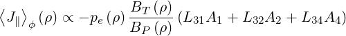
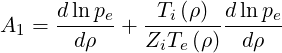
A comparison between results given by the drift kinetic code and well known analytical expressions that may be found in Refs. [?][?][?][?][?][?] is performe. For Maxwellian plasmas circular magnetic flux surfaces, in the low aspect ratio limit ϵ → 0 and low collisionality limit ν* → 0, flux surface-averaged parallel current may be expressed in the general simple form
 | (7.15) |
where
 | (7.16) |
 | (7.17) |
 | (7.18) |
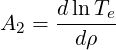
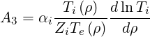
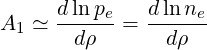
pe being the electron pressure. Neoclassical transport coefficients L31, L32 and L34 and the parameter αi depends of the model. For the non-relativistic Lorentz model, with flat temperature gradients, A2 = A3 = 0, and consequently only the coefficient L31 plays a role. Therefore both models [?] and [?] are expected to give equivalent results. Moreover since Zi ≫ 1 and Ti∕Te ≪ 1,
 | (7.19) |
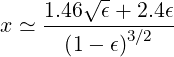
In the low collisionality limit but for arbitrary inverse aspect ratio between 0 and 1, the expression of L31 given by Hirshman [?] may be used
![L = x[0.754+ 2.21Z + Z2
31 ( i i 2)]
+ x 0.348 + 1.243Zi + Z i ∕D (x) (7.20)](NoticeDKE4326x.png)

 | (7.22) |
In the limit Zi ≫ 1,
 | (7.23) |
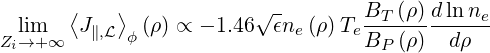
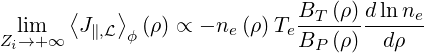
L31 is independent of Zi. Therefore, the flux-surface averaged bootstrap current scales as
 | (7.24) |
with
 | (7.25) |
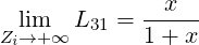
and using the definition pe ≡ neTe. For the case here studied, Rp ≈ ap and consequently ρ = ϵ. With the expression (7.24), the well known limit ϵ ≪ 1
 | (7.26) |
is recovered, while
 | (7.27) |
when ϵ → 1.9
As shown in Fig.7.44, the agreement between the bootstrap current calculated by the
code and determined by the Hirshman or Sauter models is excellent for all ρ values
10. The
model given in Ref. [?] strongly fails, since it corresponds only to the case Zi = 1.
A confirmation of the robustness of the code is the very good agreement between
numerical caclualtions and analytical expressions of the effective trapped fraction
 teff.
teff. at all plasma radii, as shown in Fig. 7.45, despite the fact that the integral
∫
-11σH
at all plasma radii, as shown in Fig. 7.45, despite the fact that the integral
∫
-11σH ξ0I
ξ0I
 dξ0 is fairly difficult to evaluate numerically, since I
 is itself an integral, as discussed in Sec. 5.6.2. A small departure is observed for the largest ϵ
value, since in that case ∫
-11σH
is itself an integral, as discussed in Sec. 5.6.2. A small departure is observed for the largest ϵ
value, since in that case ∫
-11σH ξ0I
ξ0I dξ0 ≃ 0, and its numerical evaluation
may have a large error on the chosen numerical grid.
dξ0 ≃ 0, and its numerical evaluation
may have a large error on the chosen numerical grid.
cmcmcm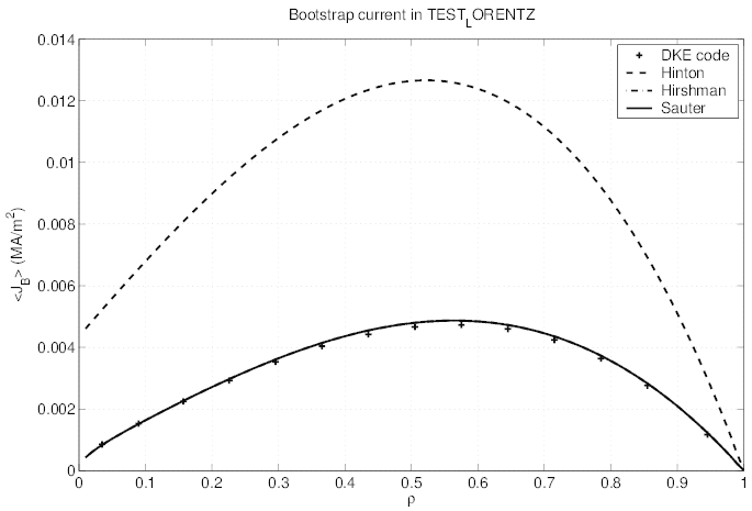
cmcmcm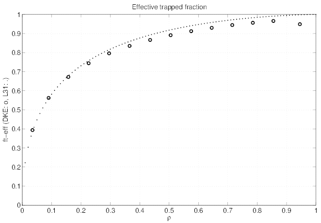
The exact trapped fraction t calculated by the code is increasing smoothly from 0 to 1 with
a radial dependence that is very different from teff. which should scale as L31 in the
simulation here studied. At the lowest ϵ ≈ 0.034 value determined by the code, the ratio
teff.
which should scale as L31 in the
simulation here studied. At the lowest ϵ ≈ 0.034 value determined by the code, the ratio
teff. ∕t ≈ 2 is larger than the expected value 1.46∕0.9 ≈ 1.62, which indicates that the
well known limit value teff.
∕t ≈ 2 is larger than the expected value 1.46∕0.9 ≈ 1.62, which indicates that the
well known limit value teff. ≃ 1.46
 is only only valid for very small inverse aspect ratio ϵ.
Indeed, t is very well reproduced by the asymptotic expression t
is only only valid for very small inverse aspect ratio ϵ.
Indeed, t is very well reproduced by the asymptotic expression t ≃ 0.9
≃ 0.9 quite far from
the limit ϵ ≪ 1, as presented in Fig.7.46. There is also very good confidence in the simulation
results since teff.
quite far from
the limit ϵ ≪ 1, as presented in Fig.7.46. There is also very good confidence in the simulation
results since teff. ≃ L31 is well verified numericaly, as expected from Hirshman
theory.
≃ L31 is well verified numericaly, as expected from Hirshman
theory.
cmcmcm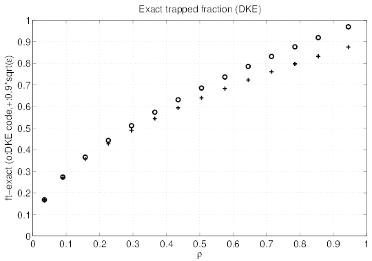
At ρ ≃ ϵ ≤ 0.4354, and for p = 4.08, the agreement for  (0) and g
 is excellent for all ξ0
values, as seen in Fig 7.47. The difference is so small between the code and the analytical
expressions given in Sec. 5.6.2, that it cannot be identify on the figure.
is excellent for all ξ0
values, as seen in Fig 7.47. The difference is so small between the code and the analytical
expressions given in Sec. 5.6.2, that it cannot be identify on the figure.
cmcmcm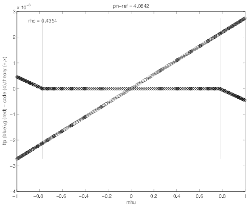
 (0) and g
 at ρ ≃ 0.4354 , as given by the drift
kinetic code and analytical expressions, for the Lorentz model limit
at ρ ≃ 0.4354 , as given by the drift
kinetic code and analytical expressions, for the Lorentz model limit
This excellent agreement is confirmed for first order distribution F∥0 averaged over the
perpendicular momentum direction p⊥
averaged over the
perpendicular momentum direction p⊥
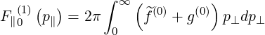 | (7.28) |
as shown in Fig. 7.48.
cmcmcm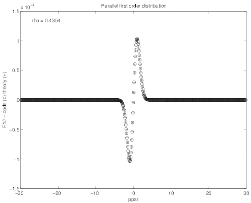
 averaged over the perpendicular momentum
direction p⊥ as fonction of p∥ at ρ ≃ 0.4354 , as given by the drift kinetic code and
analytical expressions, for the Lorentz model limit
averaged over the perpendicular momentum
direction p⊥ as fonction of p∥ at ρ ≃ 0.4354 , as given by the drift kinetic code and
analytical expressions, for the Lorentz model limit
In Figs. 7.49 and 7.50, the 2-D contour plot of  (0) and g
 are represented. As expected for
a Maxwellian distribution function, g
are represented. As expected for
a Maxwellian distribution function, g = 0 in the trapped region while
  (0) is clearly
antisymmetric.
(0) is clearly
antisymmetric.
cmcmcm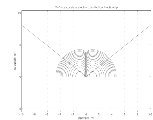
 (0) at ρ ≃ 0.4354 , as given by the drift kinetic code for the
Lorentz model limit
(0) at ρ ≃ 0.4354 , as given by the drift kinetic code for the
Lorentz model limit
cmcmcm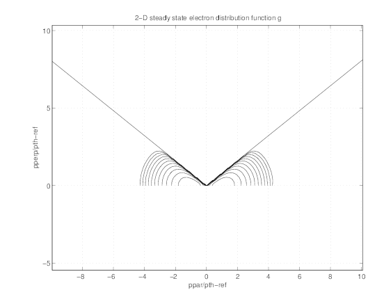
 at ρ ≃ 0.4354 , as given by the drift kinetic code for the
Lorentz model limit
at ρ ≃ 0.4354 , as given by the drift kinetic code for the
Lorentz model limit
The overall results confirm that the drift kinetic solver gives the correct dependences and level of the first order neoclaissicla corrections. The robustness of the code is remarkable, since no specific boundary conditions have to be imposed at the limits of the domain to ensure the determination of the correct solution.
The Maxwellian bootstrap current for a realistic tokamak magnetic configuration has been calculated. Here the Tore Supra tokamak is studied, with numerical parameters that are similar to the case of the discussed in the previous section, while physical parameters, in particular pressure profiles, are those taken for magnetic ripple losses studies (see Sec. 7.6). The full first order Legendre collision term for momentum conservation is now considered, which is crucial to estimate the right current level.
As shown in Fig. 7.51, an excellent agreement with both Hirschman and Sauter models given in Refs. [?] and [?] is found at plasma radii. In that case the maximum inverse aspect ratio reaches approximately 0.3. The Hinton model fails also, since an effective charge Zeff = 1.5 is considered, the major light impurity being fully strip carbon.
cmcmcm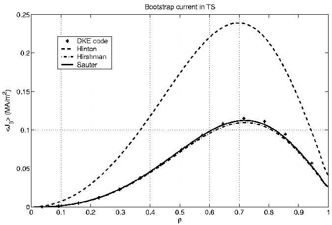
The exact t and effective teff.
 trapped fraction are given respectively in Figs. 7.52
and 7.53. In that case, the exact trapped fraction reaches t
trapped fraction are given respectively in Figs. 7.52
and 7.53. In that case, the exact trapped fraction reaches t ≃ 0.5 at the edge, while the
effective one teff.
≃ 0.5 at the edge, while the
effective one teff. ≃ 0.7. This difference may be easily understood, since in the calculation
of the effective trapped fraction, the time spend on the banana orbit is considered, while it is not
for the exact trapped fraction.
≃ 0.7. This difference may be easily understood, since in the calculation
of the effective trapped fraction, the time spend on the banana orbit is considered, while it is not
for the exact trapped fraction.
For the exact trapped fraction, the level at the limit ϵ ≪ 1 is very consistent with
the analytical expression given in Sec.3.6. A very good agreement is also found for
teff. given by the HELENA equlibrium code using the analytical formula (see also
Sec.3.6).
given by the HELENA equlibrium code using the analytical formula (see also
Sec.3.6).
cmcmcm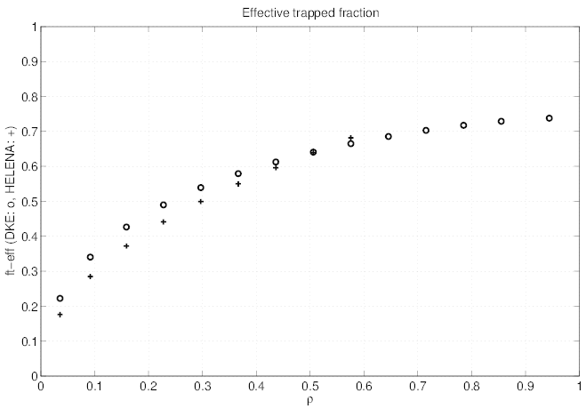
cmcmcm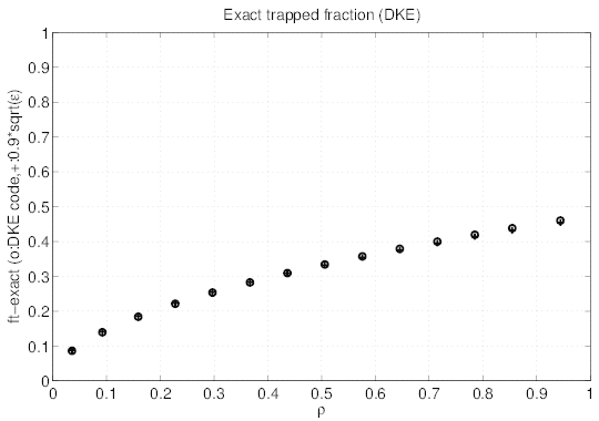
As for the case of the Lorentz model, the pitch-angle dependence at ρ = 0.435 and for
p = 4.08 of first order distribution functions  (0) and g
 is given as function of ξ0. Similar
dependences are observed in Fig 7.54 as well as for the first order distribution F∥0
is given as function of ξ0. Similar
dependences are observed in Fig 7.54 as well as for the first order distribution F∥0 averaged
over the perpendicular momentum direction p⊥ shown in Fig. 7.55
averaged
over the perpendicular momentum direction p⊥ shown in Fig. 7.55
cmcmcm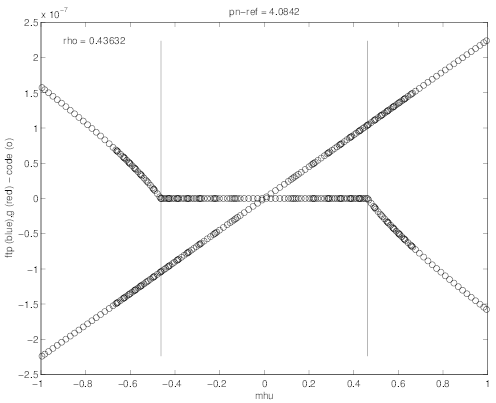
 (0) and g
 at ρ ≃ 0.4354 , as given by the drift
kinetic code for the tokamak Tore Supra
at ρ ≃ 0.4354 , as given by the drift
kinetic code for the tokamak Tore Supra
cmcmcm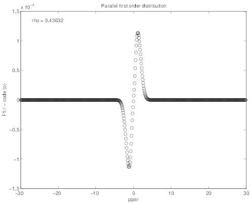
 averaged over the perpendicular momentum
direction p⊥ as fonction of p∥ at ρ ≃ 0.4354 , as given by the drift kinetic code for the
tokamak Tore Supra
averaged over the perpendicular momentum
direction p⊥ as fonction of p∥ at ρ ≃ 0.4354 , as given by the drift kinetic code for the
tokamak Tore Supra
In Figs. 7.56 and 7.57, the 2-D contour plot of  (0) and g
 are represented. As expected for
a Maxwellian distribution function, g
are represented. As expected for
a Maxwellian distribution function, g = 0 in the trapped region while
  (0) is clearly
antisymmetric.
(0) is clearly
antisymmetric.
cmcmcm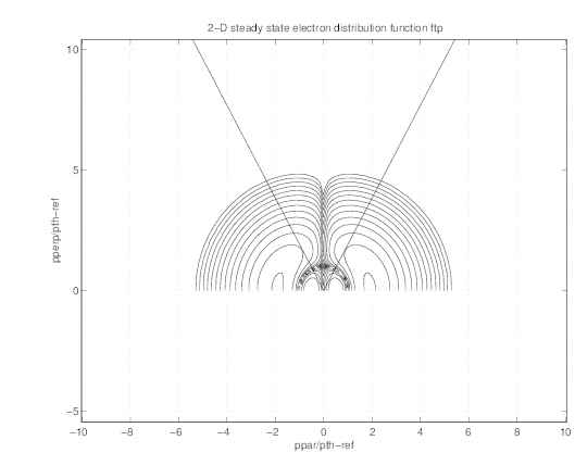
 (0) at ρ ≃ 0.4354 , as given by the drift kinetic code for the
tokamak Tore Supra
(0) at ρ ≃ 0.4354 , as given by the drift kinetic code for the
tokamak Tore Supra
cmcmcm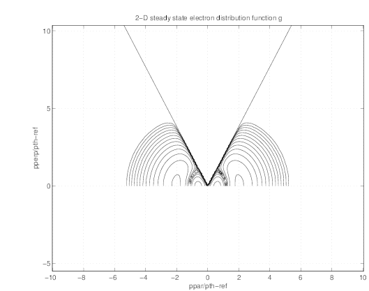
 at ρ ≃ 0.4354 , as given by the drift kinetic code for the
tokamak Tore Supra
at ρ ≃ 0.4354 , as given by the drift kinetic code for the
tokamak Tore Supra
These results illustrate that the drift kientic code is able to determine accurately the boostrap current level. For the ion contribution, the expression given in the fluid limit as given in Ref. [?] is taken. This is the same value taken in Ref. [?], only the coefficent L32 being different. However, for this case, results are very similar, though the drift kinetic code results seem more closer to the one given by the Sauter formula [?][?].