6.2 Inversion procedure

6.2.1 Incomplete matrix factorization

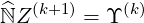
According to Sec. 6.1.1, the electron Fokker-Planck equation may be expressed in a general symbolic matrix form

(6.12)

where Z = X with

The formal expression (6.12) may be also used for the electron drift kinetic equation as shown in Sec. 6.1.2, and in this case, Z = Y with

In all cases, matrices are square with similar structures, i.e. non-zero elements are aligned along a reduced number of diagonals which are roughly symmetricaly placed around the main one⁴, as shown in Fig.6.3. Consequently, the method for determining the asymptotic solution

cmcmcm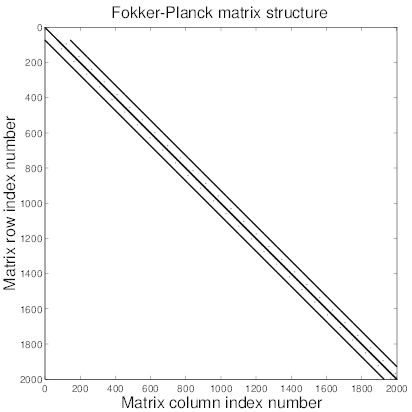

Figure 6.3: Typical arrangement of non-zero matrix coefficients in the first 2000 columns and rows in matrix corresponding to the Fokker-Planck equation

(6.19)

of the system of equations (6.12) will be the same, either for the Fokker-Planck or the drift kinetic equations.

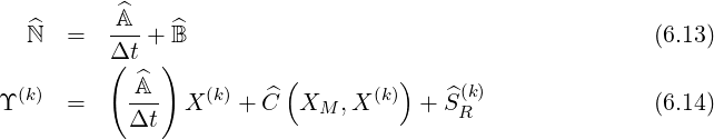
In order to avoid manipulation of large matrix coefficients that may reduce the numerical accuracy and also leads often to numerical instabilities, main diagonal matrix preconditioning is first performed. The modified system of equation to solve is then

(6.20)

where all the coefficients of the main diagonal of matrix ^′

(6.21)

are one by definition. Here _N is a diagonal matrix whose coefficients are those of the main diagonal of . Since collision is the dominant physics process, all off-diagonal coefficients are usualy less than one, as shown in Fig.6.4, except when specific internal boundary conditions apply, like at ξ₀ = 0 in the trapped region.

cmcmcm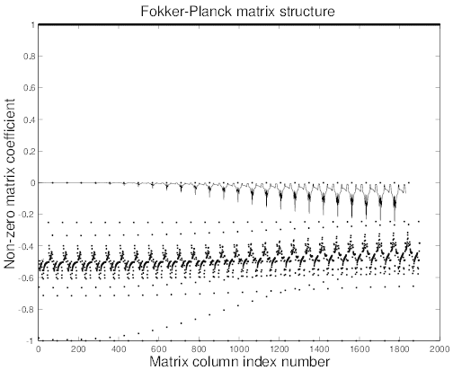

Figure 6.4: Values of the non-zero matrix coefficients after diagonal preconditionning for matrix ^′ corresponding to the Fokker-Planck equation. Dot points correspond to pitch-angle process at constant p, while full line for slowing-down process at constant ξ₀. By definition values of all coefficients on the main diagonal are one

The determination of Z^(k+1) requires to invert the system of equation (6.12). The usual method based on a direct inversion by the well known Gaussian elimination is immediately ruled out, since the number of operations for each direction is , where N is the number of rows (or columns) of matrix . For the example n_ψ = 20, n_p = 200 and n_ξ0 = 200 discussed in Sec. 6.1.1, N = n_ψn_pn_ξ0 = 800000, ≃ 10⁺¹⁷, corresponding to a prohibitive number of operations. In addition, since memory requirements grow as unacceptable storage constraints take also place.

Consequently, alternative methods must be used, in order to perform a fast matrix inversion without the need of a large memory storage requirement. The basic principle is to factorize ^′ into upper and lower triangular matrices and respectively

(6.22)

as shown in Fig. 6.5, that are themselves highly sparse matrices. A strong reduction of the computational effort may then be foreseen, since the number of coefficients that are considered in the calculations is considerably lower. Indeed, aside from the time required to perform the matrix factorization itself which represents a computational effort equivalent to a direct matrix inversion, each further inversion needs only operations for each triangular system of equations as shown in the next sections. Therefore, for large values of N, a substantial gain may be expected, as soon as the number of iterations for an accurate estimate of the solution Z^(∞) is greater than unity. This is usually the case for the time dependent problem where all time steps must be evaluated, but also when only the steady-state solution Z^(∞) is seeked, since the non-linearity resulting form self-collision operators requires several iterations either for the Fokker-Planck or the drift kinetic equations. This elegant approach has been first considered for Fokker-Planck calculations for a five diagonals operator as presented in Ref. [?], since in that case and are both triangular and tridiagonal matrices. However, as discussed in Ref. [?], the fact that cross-derivatives are considered explicitely with respect to the time differencing scheme puts strong limitations. Indeed, the integration time step Δt must be much lower than one for an accurate determination of the solution of the set of linear equations. Consequently, the overall time duration for calculating the steady-state solution is very long, an important drawback when the kinetic solver must be incorporated in a chain of codes for realistic tokamak simulations.

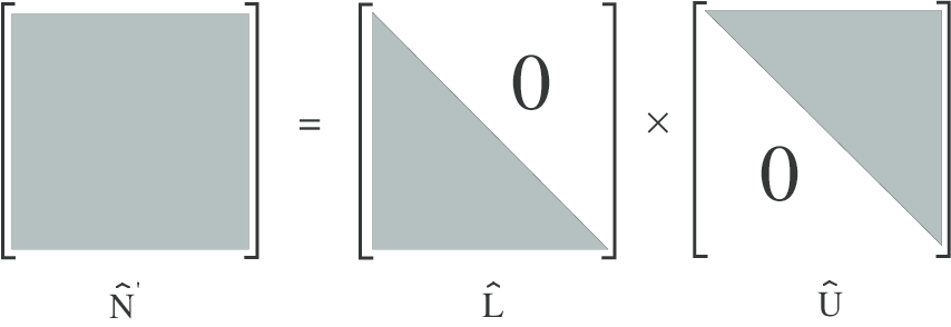
For this purpose, this method has been succesfully extended to the nine diagonals operator case, allowing the use of much larger Δt values while the numerical scheme remains stable, as shown in Ref. [?]. However, this approach is only useful for local kinetic calculations, where trapped particle contribution is negligible, i.e. close to the plasma center. When off-axis electron dynamics must be described, one must in that case fully consider both circulating and trapped electron dynamics which leads to a number of diagonals with non-zero elements that is much larger, fifteen diagonals at each radial location as shown in Fig. 6.1. Therefore, the method developped for nine diagonal operators may no more be used, since the number of operations to determine and increases dramaticaly. The fully 3 - D approach with radial transport makes also this method unusable, since the matrix that must be inverted has no more the nine diagonal structure.

However, an equivalent form of the approximate matrix factorization may still be employed, noting that exact and matrices are made of a large number of very small coefficients, close to zero. This indicates that information on the electron dynamics is fully contained in a few set of coefficients, whose number is several order of magnitude lower than the total one. Such a structure results in fact from the well conditionning of the matrix ^′, a physical consequence that collisions predominate over all other physical processes. Consequently, the general approach is to introduce a non-negative scalar named as the drop tolerance parameter δ_lu, below which small coefficients of exact and matrices are forced to zero. By this way, an approximation of the exact matrix factorization is performed. The only exception to the dropping rule is the diagonal of the upper triangular matrix which is preserved even if coefficients are too small, in order to avoid singular factors. Since coefficients of ^′ lie between 0 and 1 in the limit where the model holds, because of the main diagonal preconditioning, the drop tolerance parameter δ_lu may be arbitrarily chosen in the same interval, i.e.

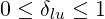(6.23)

and when δ_lu is close to 0, approximate and exact matrices and are roughly equivalent, while they differ strongly when δ_lu tends to one. In the latter case, considerable saving may be foreseen for the memory requirement, as well as a significant reduction of the computer time consumption, since less non-zero coefficients must be considered. An example is shown in Fig. 6.6, where δ_lu varies from zero to 10^-2. Consequently, from the exact matrix factorization to the approximate one, the number of non-zero elements drops by a factor around 30.

cmcmcm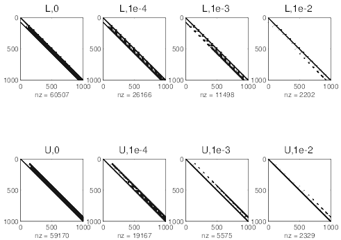

Figure 6.6: Reduction of the non-zero elements for the and matrices, by increasing δ_lu. Values of δ_lu are indicated on the top of each subfigure. For δ_lu = 10^-2, the inversion becomes instable.

The rule is therefore to find the largest δ_lu value that is compatible with a stable inversion procedure, even in presence of a large Ohmic electric field or a high RF power. However too large δ_lu values will remove important physical informations, leading to spurious solutions. However, it turns out that margins are usually considerable, making the method very effective. An example is given in Fig. 6.7, which illustrates the effectiveness of the method, for the Lower Hybrid current drive local problem. For δ_lu ≃ 2 × 10^-3, memory size requirement to store matrices and does not exceed 2.2MBytes, while it reaches 66MBytes when δ_lu = 0. It is interesting to observe that the convergence rate towards the steady-state solution Z^(∞) is reduced by 50%, and that the result is moreover independent of δ_lu. For larger δ_lu values, the inversion scheme becomes progressively unstable, and the benefit gains on the memory storage requirement is therefore cancelled by a reduced rate of convergence. For this reason, the upper value used in the code is usually δ_lu ≃ 2 × 10^-3. More refined methods may be used to optimized the choice of δ_lu. The trade-off that must be found between memory saving and stability of the inversion procedure requires extensive investigations that are beyond the scope of this document. Hopefully, it turns out that the domain 1 × 10^-4 ≤ δ_lu ≤ 2 × 10^-3 covers must of the parameter range for the current drive problem in tokamaks, even in presence of radial transport. Since the local problems needs only 2.2MBytes, it is therefore possible to extrapolate that the full 3 - D problem with 20 radial positions will only require approximately 44MBytes. This result has justified the development of this new approach.

6.2.2 Zero order term: the Fokker-Planck equation

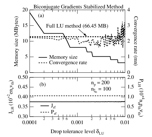
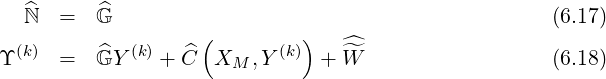
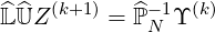
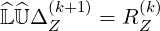
The matrix inversion procedure is based on the possibility of matrix factorization as discussed in Sec.6.2.1. Formally, the iterative method may be expressed in the simple form

(6.24)

where β_C is the iteration parameter that may be adjusted for an improvement of the rate of convergence, using a Chebyshev acceleration technique as shown in Ref. [?]. Here is used for the main diagonal precondiotiong as explained in Sec.6.2.1 . However, it has been shown that values of β_C other than unity do not give much better results in general for implicit methods ([?]), and therefore, only the case β_C = 1 is considered. Then Eq. 6.24 is equivalent to Eq. 6.12 given in Sec. 6.2.1. Replacing ^′ by , one obtains

(6.25)

If we introduce the increment Δ_Z^(k+1)

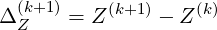(6.26)

and the residual R_Z^(k)

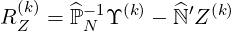(6.27)

Eq.6.25 becomes simply

(6.28)

which can be solved by two successive inversion steps, evaluating respectively forward and backward solutions from triangular systems of equations

For achieving convergence towards the steady state solution Z^(∞), various iterative methods may be used, like the Conjugate Gradient Squared (CGS), the BiConjigate Gradient (BICG) or the Quasi-Minimal Residual (QMR) methods. These methods, which both give equivalent results in term of convergence rate, are preferred to the BiConjigate Gradient Stabilized (BICGSTAB) method, since the conservative scheme is nearly always well fullfiled even for marginaly well-conditionned matrices, like in presence of RF waves whose intensity is large. All methods here considered are build-in MatLab functions whose principle may be found in Refs. [?] or [?] for more detailed insights.

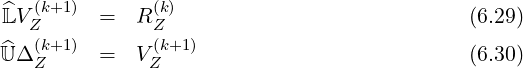
After numerous tests, it has been found that the drop tolerance parameter δ_lu has a close link with the maximum number of iterations MAXIT allowed inside the function that performs the iterative matrix inversion, in order to avoid cumulative numerical errors that lead usually to violation of the conservative nature of the code. Even if this problem may be cured by forcing the Maxwellian solution close to p = 0 and normalizing the solution at each iteration, this approach has not been considered, because it may hinder more serious problems regarding the overall numerical conservative scheme. So far, a very robust and fully conservative scheme is achieved with the following rule of thumb

(6.31)

for all cases addressed by the code, including the in presence of RF waves. More detailed studied are necessary to clarify this point.

At each iteration, Z^(k+1) is evaluated from the knowledge of Δ_Z^(k+1), and the electron distribution function f_{0,l+1∕2,i+1∕2,j+1∕2} is reconstructed in order to evaluate the non-linear term that arises from self-collisions. Though this procedure is quite time consuming, its incidence on the overall time for converging is fairly marginal, since the number of iterations never exceeds 10 in most cases.

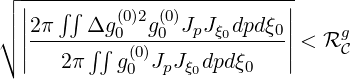
According to Ref. [?], convergence towards Z^(∞) is considered to be achieved and the iteration is stopped when the following criterion is fullfiled

(6.32)

for an arbitrarily small ^f, at all plasma locations ψ, where J_p and J_ξ0 are the partial Jacobians as introduced in Sec. 3.5.1⁵.

Projected on the numerical grid, the criterion (6.32) becomes

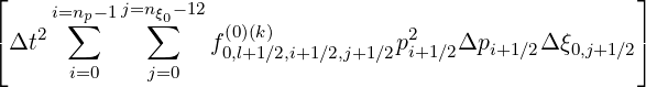	1∕2
	×-1∕2
	< f	(6.33)

The criterion introduced in Ref. [?] has the main advantage to ensure that convergence is achieved not for electrons whose energy is close to the thermal one, but also for the fastest when a tail is driven by an external source. Usually, ^f ranges between 10^-10 and 10^-12, and in the code the standard value is 10^-11. The quantity (6.32) may be viewed as a norm, and its definition is consequently independent of the level of current which results from the the lack of symmetry of f₀ in momentum space. It may therefore be used for strong deformations of the electron distribution function, even if the net current is close to zero.

In practice, the total number of iteration ^f is a free choice. It is usually set to 50, so that inversion procedure stops when (6.32) is fullfiled in quite all cases. If the number of iterations reaches ^f, the program warns that convergence is not achieved and that something is going wrong in the calculations. This may occur sometimes when too large quasilinear RF diffusion coefficient are used, leading to inconsistent and non physical solutions. This point is extensively discussed in Sec.7.3. Conversely, when time step is very large, i.e. Δt ≥ 1000, the convergence may be achieved for a given value ^f before the current level is fully established. Such an event may arise because there is a too reduced number of iterations which involves the 1^st order Legendre non-linear correction term for momentum conservation. Consequently, to avoid this problem, a minimum number of iterations has been set to 6, which turns out to be enough for giving reliable results, owing to the weakness of the non-linearity.

6.2.3 Up to first order term: the Drift Kinetic equation

The inversion procedure for solving the first order drift kinetic equation is exactly similar to the one described in Sec. 6.2.2. Indeed, the linear system of equation to be solved may be cast in a similar form. Usually, the convergence coefficient ^g is set to similar values than for the Fokker-Planck problem, while the maximum number of iterations allowed ^g is slightly larger ⁶, since the convergence requires more iterations, around 20 - 30. Since the function g₀ may be negative and that dt has no sense here, as the solution is determined once the steady-state regime is achieved, the convergence criterion is modified accordingly

(6.34)

at all plasma locations ψ. Here again J_p and J_ξ0 are the partial Jacobians introduced in Sec. 3.5.1⁷.

Projected on the numerical grid, the criterion (6.34) becomes

	1∕2
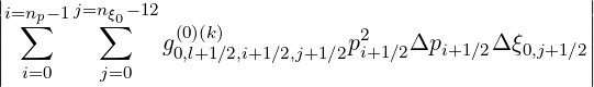	×-1∕2 < g	(6.35)

where is the iteration step number. Since all quantities are normalized, this definition is fully acceptable. If the number of iterations reaches ^g, the program warns that convergence is not achieved and that something is going wrong in the calculations, as for the Fokker-Planck part.