.
.
General and specific properties of curvilinear coordinate systems are detailed in Appendix A. In
this work, vectors are written in bold characters, like v, except unit vectors, which are covered
with a hat, like .
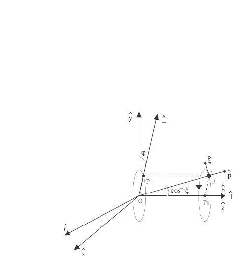
Because we consider gyro-averaged kinetic equations, it is important to use coordinates with rotational symmetry in order to reduce the dimensionality of the problem. Two different momentum space coordinates system are considered here:
 , where p∥ is the component of the
momentum along the magnetic field, and p⊥ is the component perpendicular and φ is the
gyro-angle. This system is defined in (A.212) and shown in Fig. 2.1. The cylindrical
coordinate system is the natural system for wave-particle interaction, or also the effect of
the electric field.
, where p∥ is the component of the
momentum along the magnetic field, and p⊥ is the component perpendicular and φ is the
gyro-angle. This system is defined in (A.212) and shown in Fig. 2.1. The cylindrical
coordinate system is the natural system for wave-particle interaction, or also the effect of
the electric field.  , where pis the magnitude of the
momentum, and ξ is the cosine of the pitch-angle. This system is defined in (A.247) and
shown in Fig. 2.1 as well. The spherical coordinate system is the natural system for
collisions. It is the primary system, used in the Drift Kinetic code, for an accurate
description of collisions.
, where pis the magnitude of the
momentum, and ξ is the cosine of the pitch-angle. This system is defined in (A.247) and
shown in Fig. 2.1 as well. The spherical coordinate system is the natural system for
collisions. It is the primary system, used in the Drift Kinetic code, for an accurate
description of collisions.
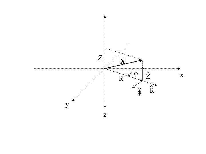
The particular toroidal geometry of tokamaks requires to use specific coordinates, in order to make use of symmetry properties such as axisymmetry, and takes into account the flux-surface magnetic configuration. Three different configuration space coordinates systems are considered here:
 , where R is the distance from the
axis of the torus, and Z the distance along this axis . This coordinates system and
the corresponding local orthogonal basis vectors
, where R is the distance from the
axis of the torus, and Z the distance along this axis . This coordinates system and
the corresponding local orthogonal basis vectors  are defined in (A.61) and
shown in Fig. 2.2. This coordinate system conserves the largest generality in the
magnetic geometry.
are defined in (A.61) and
shown in Fig. 2.2. This coordinate system conserves the largest generality in the
magnetic geometry.
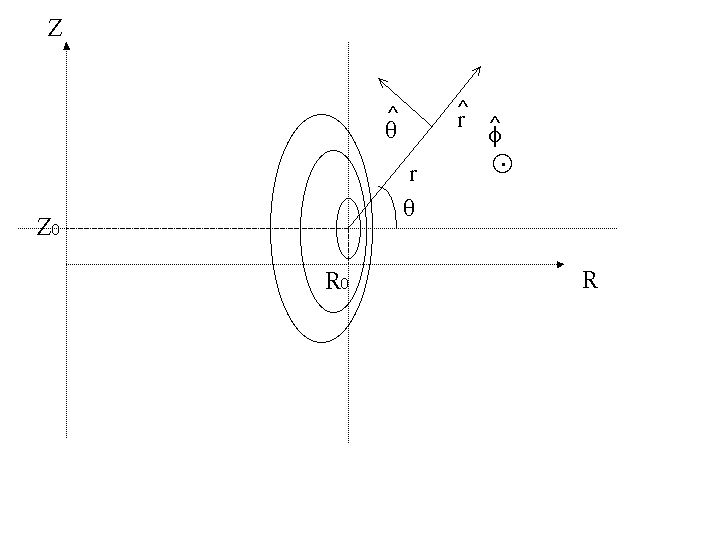
 assumes the existence of a toroidal
axis at constant position
assumes the existence of a toroidal
axis at constant position  which is typically the plasma magnetic axis,
corresponding to the position of an extremum of the poloidal magnetic flux ψ (which can
be arbitrarily chosen as ψ = 0). This coordinates system and the corresponding
local orthogonal basis vectors
which is typically the plasma magnetic axis,
corresponding to the position of an extremum of the poloidal magnetic flux ψ (which can
be arbitrarily chosen as ψ = 0). This coordinates system and the corresponding
local orthogonal basis vectors  are defined in (A.94) and shown in Fig.
??.
are defined in (A.94) and shown in Fig.
??.
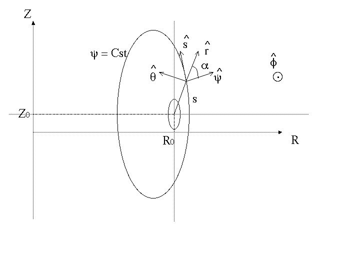
 is the natural system when we describe
particles which are confined to a given flux surface ψ. This coordinates system and the
corresponding local orthogonal basis vectors
is the natural system when we describe
particles which are confined to a given flux surface ψ. This coordinates system and the
corresponding local orthogonal basis vectors  are defined in (A.136) and shown in
Fig. 2.4
are defined in (A.136) and shown in
Fig. 2.4
. The vector  is perpendicular to the flux surface, while
  is parallel to the surface, and
included in the poloidal plane. The distance s is the length along the poloidal magnetic
field lines. We can choose its origin as being at the position of minimum B-field amplitude
within a flux-surface.
is parallel to the surface, and
included in the poloidal plane. The distance s is the length along the poloidal magnetic
field lines. We can choose its origin as being at the position of minimum B-field amplitude
within a flux-surface.
 | (2.1) |
Note that from now on, and all along this paper, the subscript 0 refers to quantities
evaluated at the position of minimum B-field on a given flux-surface. The direction of
evolution of s is counter-clockwise and the limits smin and smax
 are set at the
position of maximum magnetic field
are set at the
position of maximum magnetic field
 | (2.2) |
 is an alternative to the previous system, which is used to implement
numerically the calculation of the bounce coefficients. One advantage is that the θ grid is
now independent of ψ, which simplifies the numerical calculations. On the other
hand, the contravariant vectors ∇ψ and ∇θ are not orthogonal, and therefore
are not respectively colinear with the covariant vectors ∂X∕∂ψ and ∂X∕∂θ.
The properties of this curvilinear system are detailed in Appendix A. We also
define, for geometrical purposes, a flux-function ρ
is an alternative to the previous system, which is used to implement
numerically the calculation of the bounce coefficients. One advantage is that the θ grid is
now independent of ψ, which simplifies the numerical calculations. On the other
hand, the contravariant vectors ∇ψ and ∇θ are not orthogonal, and therefore
are not respectively colinear with the covariant vectors ∂X∕∂ψ and ∂X∕∂θ.
The properties of this curvilinear system are detailed in Appendix A. We also
define, for geometrical purposes, a flux-function ρ which coincides with the
normalized radius on the horizontal Low Field Side (LFS) mid-plane. Indeed, in an
axisymmetric system, using the functions R
which coincides with the
normalized radius on the horizontal Low Field Side (LFS) mid-plane. Indeed, in an
axisymmetric system, using the functions R and Z
and Z , we define ρ
 as
as
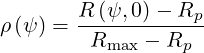 | (2.3) |
with 0 ≤ ρ ≤ 1 by construction, and where Rmax = R is the value of R on the
separatrix as it crosses the mid-plane. Here ap = Rmax - Rp is defined arbitrarily as the
plasma minor radius since this definition merges with the exact one for circular
concentric flux-surfaces. The 2 - D outputs from the axisymmetric equilibrium code
HELENA are given on the
is the value of R on the
separatrix as it crosses the mid-plane. Here ap = Rmax - Rp is defined arbitrarily as the
plasma minor radius since this definition merges with the exact one for circular
concentric flux-surfaces. The 2 - D outputs from the axisymmetric equilibrium code
HELENA are given on the  grid [?]. The system
  will be used from now
on.
will be used from now
on.
 and
and  for momentum dynamics