
Analytic expression for the properties of LH waves can be obtained in the cold plasma description if further approximations are made. Then, an analytical expression can be obtained for the LH diffusion coefficient.
We consider the wave equation (D.4)
|
| (D.31) |
The electric field can be separated into its longitudinal and transverse components with respect to the normalized wave vector Nb:
 | (D.32) |
so that the wave equation (D.31) becomes
 | (D.33) |
Electrostatic waves, and also electromagnetic waves approaching resonances, such as LHW, can satisfy the condition
 | (D.34) |
and therefore (D.33) reduces to
 | (D.35) |
Dot-multiplying (D.35) by  b = Nb∕Nb leads to the electrostatic dispersion relation
 | (D.36) |
and the transverse electric field is given by
 | (D.37) |
We note from (D.37) and (D.34) that |EbT |≪|EbL|. The electric field is quasi longitudinal, which justify the term electrostatic approximation given to the condition (D.34).
Using (D.6), the electrostatic dispersion relation (D.36) in the cold plasma limit is then given by
 | (D.38) |
which gives an expression for Nb⊥ as a function of Nb∥ and ωb:
 | (D.39) |
We consider the lower-hybrid range of frequency in a electron-ion plasma, where the following ordering applies
 | (D.40) |
Assuming in addition that
 | (D.41) |
leads to approximate expressions of the dielectric tensor components given by:
| K⊥ | ≃ 1 +  - - | ||
| K∥ | ≃- | (D.42) | |
| Kxy | ≃ | (D.43) |
where K⊥ can be rewritten as
| K⊥ | =   | (D.44) |
=   | (D.45) | |
=   | (D.46) |
where
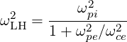 | (D.47) |
is the lower hybrid frequency.
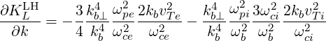
The perpendicular index of refraction becomes
 | (D.48) |
We recognize that Nb⊥ →∞ as the the lower-hybrid frequency approaches the wave frequency. However, in most LHCD scenarios, wave frequency are sensibly higher than the lower-hybrid frequency in order to avoid conversion to IBW. Typically, in Alcator C-Mod, we have
 | (D.49) |
In that case, and as shown in D.2.7, the contribution of ΦbT to the power flow can be neglected. The cold plasma description therefore remains valid.
The LH Waves of concern for LHCD are quasi-electrostatic, and therefore the electric field is quasi-longitudinal (Eb ∥ Nb) and we have
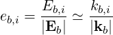 | (D.50) |
for any component i, so that the polarization elements become
| eb,+ | ≡ = =   = =  e+iα e+iα | (D.51) | |
| eb,- | ≡ = =   = =  e-iα e-iα | ||
| eb,∥ | ≡ = =  |
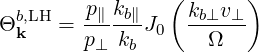
Lower Hybrid Current Drive (LHCD) results from momentum exchange from the LH wave to the plasma through Landau damping (harmonic n = 0). In this case, the coefficient (4.308) becomes
| Θkb,0 | =  eb,+e-iαJ
-1 eb,+e-iαJ
-1 + +  eb,-e+iαJ
1 eb,-e+iαJ
1 + +  eb,∥J0 eb,∥J0 | (D.52) |
=   J
1 J
1 + +  eb,∥J0 eb,∥J0 | (D.53) |
Using (D.51), we see that the perpendicular components cancel and we are left with
 | (D.54) |
The argument of the Bessel function in (D.54) is
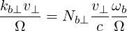 | (D.55) |
where an expression for N⊥ is given by (D.48). The argument of the Bessel function becomes
 | (D.56) |
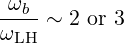
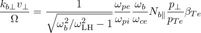
and we see that for ωpe ~ ωce and ωb ~ 2ωLH, we get
 | (D.57) |
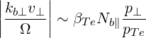
Given that most electrons concerned with LHCD have p⊥~ pTe, and that for LHCD we have typically Nb∥~ 2, we see that it is reasonable to take the limit
 | (D.58) |
as long as the plasma is not too relativistic (βTe ≪ 1). This limit is consistent with the validity condition of the cold plasma description. In this limit, valid for most LHCD scenarios, we have
 | (D.59) |
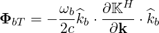
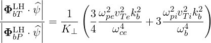
The vector ΦbLH describes the relation between the energy flux and the electric field. Although LHW are almost electrostatic, the dominant contribution to the power flux is the wave Poynting flux ΦbP LH, assuming that the wave frequency remains sensibly higher than the LH frequency. The contribution of the Kinetic power flux is calculated in D.2.7. In most LHCD scenarios, this contribution is not more than a few percents of the total flux and can therefore be neglected. We have (D.28).
![[ 2 ]
ΦbP = Re |ebT| Nb - NbebLe *bT](NoticeDKE5230x.png) | (D.60) |
LH waves are quasi-electrostatic, so that the longitudinal and transverse components are given by (D.37)
| ebL | ≃ 1 | (D.61) |
| ebT | =  K ⋅ ebL K ⋅ ebL | (D.62) |
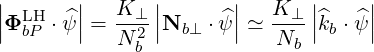
so that the first term in (D.60) can be neglected, and
| ΦbP LH | ≃ Re | ||
= Re | (D.63) |
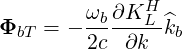
Note from (D.63) and (D.36) that the Poynting flux is in the direction perpendicular to the wave vector:
 | (D.64) |
We finally find, using (D.6),
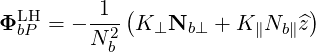 | (D.65) |
In the analysis above the kinetic part of the power flux, due to the coherent motion of charge carriers, has been neglected. This approximation must be justified by comparing the Poynting and the kinetic fluxes.
The normalized expression for the kinetic power flux associated with an electromagnetic wave in a kinetic plasma is given by (4.286)
 | (D.66) |
In the electrostatic approximation, the electric field is quasi-longitudinal (D.37)
 | (D.67) |
and (D.66) becomes
 | (D.68) |
In the frame of the wave vector  b, (D.68) can then be expressed as
 | (D.69) |
where
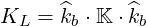 | (D.70) |
is the longitudinal (electrostatic) component of the dielectric tensor.
An expression of the electrostatic dispersion relation for LH waves that includes the first-order thermal corrections is given by [?]:
 | (D.71) |
where the finite Larmor radius (FRL) effects are scaled by the parameters
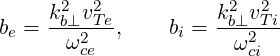 | (D.72) |
with vT 2 = T∕m.
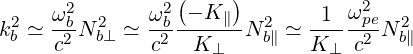
The k-dependence of the dispersion relation is found in the thermal correction terms so that
 | (D.73) |
Inside the plasma, we have kb∥2 ≪ kb⊥2 and therefore kb⊥2∕kb2 ≃ 1. We finally get the following expression for the kinetic flux associated with quasi-electrostatic LH waves:
 | (D.74) |
The kinetic flux is oriented in the direction of the wave vector, and the incident flux on the flux surface
 | (D.75) |
This incident kinetic flux must be compared to the incident Poynting flux taken in the cold plasma limit from (D.65)
 | (D.76) |
The ratio of the incident kinetic power flux to the Poynting flux is given by
 | (D.77) |
Using (D.39) we have
 | (D.78) |
so that
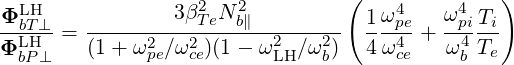 | (D.79) |
where βTe2 = Te∕mc2.
It can be seen from (D.79) that the kinetic part of the power flux becomes significant only as the wave approaches the lower-hybrid resonance very closely. In a typical LHCD context (for instance Alcator C-Mod, [?]), we have
 | (D.80) |
so that the kinetic part of the power flux is not more than a few percents.
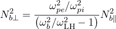
The normalized bounce-averaged diffusion coefficient for the Fokker-Planck equation is given by (4.331)
| DbLH(0)(p,ξ 0) | =      ΨθbDb,0LH,θb
× ΨθbDb,0LH,θb
× | ||
H H H ![[ ]
1-∑
2
σ](NoticeDKE5259x.png) T δ T δ  2 2 | (D.81) |
with
| Db,0LH,θb | =     Pb,inc Pb,inc | (D.82) |
| N∥resθbLH | =   | (D.83) |
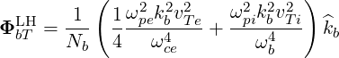
Within the electrostatic approximation and in the small FLR limit, we have obtained the following expressions for the LHW properties (D.59), (D.39), (D.65)
| Θk,θbb,LH | =   | (D.84) |
| Nb⊥ | =  Nb∥ Nb∥ | (D.85) |
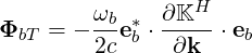
| ΦbLH | = -  | (D.86) |
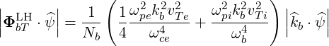
so that
 | =   | (D.87) |
≃  | (D.88) | |
=  | (D.89) |
and where K⊥ and K∥ are given by (D.44) and (D.42) respectively
We consider the limit of a large aspect ratio tokamak with circular flux-surfaces (limit of a cylindrical plasma). In that case, rθb∕Rp → 0 and the effects of magnetic trapping disppear. We can use the following asymptotic expressions
| Ψθb | → 1 | (D.90) |
λ | → 1 | (D.91) |
   | → 1 | (D.92) |
 | → 1 | (D.93) |
Because of cylindrical symmetry, the dependence θb on disappears.
The QL diffusion coefficient for LHCD (D.81) can therefore be written as
 | (D.94) |
with
| Db,0LH | =     finc,bl+1∕2P
b,inc finc,bl+1∕2P
b,inc | (D.95) |
| N∥resLH | =   | (D.96) |
and where we used Nb ≃ Nb⊥ and assume a square power spectrum as in (4.351).
In order to compare with LHCD operators found in the litterature, we redefine the LH constant factor such that
 | (D.97) |
with
| Db,0,newLH | =   Db,0LH Db,0LH | (D.98) |
=     finc,bl+1∕2P
b,inc finc,bl+1∕2P
b,inc | (D.99) |
A familiar expression for the LH QL operator is obtained in cylindrical geometry. From (4.239) and (4.242-4.245) we see that for LHCD, the QL operator can be rewritten as
| QLH(f) | =  D∥∥RF D∥∥RF | ||
= ∑
b Db,0,newLH Db,0,newLH H H H H  | (D.100) |
Although it is better to keep the exact formula (D.100), the factor vTe∕ has often been
neglected in the litterature, which is an acceptable approximation when Db,0,newLH ≫ νepTe2
and ΔNb∥≪ Nb∥ min. In this case, considering only one ray b, the LH Operator reduces
to
has often been
neglected in the litterature, which is an acceptable approximation when Db,0,newLH ≫ νepTe2
and ΔNb∥≪ Nb∥ min. In this case, considering only one ray b, the LH Operator reduces
to
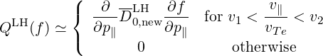 | (D.101) |
with
| v1 | =  | (D.102) |
| v2 | =  | (D.103) |
| D0,newLH | = ![[ ]
vTe
|v∥|](NoticeDKE5309x.png) Db,0,newLH Db,0,newLH | (D.104) |
=      fincl+1∕2P
inc fincl+1∕2P
inc | (D.105) |
where ![[ ]
v|T-e|
|v∥|](NoticeDKE5315x.png) is an averaged value of
is an averaged value of  which can be taken to be
  and
then
and
then
 | (D.106) |