 ≪ 1, the two modes are the
quasi-X and quasi-O modes.
≪ 1, the two modes are the
quasi-X and quasi-O modes.
The cold plasma description is usually a good approximation to determine the ECW properties, as long as we stay away from the upper-hybrid resonance, where mode-conversion to EBW occurs. However, even in the cold plasma model, the polarizations are usually mixed for oblique propagation, and no simple analytical formulation is possible. Still, it is possible to find limit cases (small FLR effects, small N∥) for which a simple analytical derivation is possible.
In the case of mostly perpendicular propagation, where ≪ 1, the two modes are the
quasi-X and quasi-O modes.
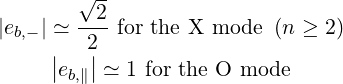
The polarization is mostly right-hand circular for X and parallel linear for O. The only exception is for the X mode near the first harmonic n = 1 where eb,-X ≃ 0. For this reason, the first-harmonic is almost transparent to the X-mode and this resonance is usually not considered. Moreover, this harmonic can only be reached from the high field side, because of the right-hand cut-off. From now, we consider only the X mode with n ≥ 2.
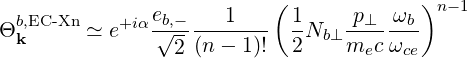
Electron Cyclotron Current Drive (ECCD) results from momentum exchange from the EC wave to the plasma through electron cyclotron damping at some harmonic n. For a ray b, considering a given harmonic n, the coefficient (4.308) is
 | (D.107) |
where zb = kb⊥v⊥∕Ω.
Since the resonance condition is ωb - kb∥v∥- nΩ = 0 and
 | (D.108) |
the only harmonics to be considered for electrons are for
 | (D.109) |
Applying the substitution
 | (D.110) |
and renaming n′→ n ≥ 0, we get
| Θkb,ECn | =  eb,+e-iαJ
-n-1 eb,+e-iαJ
-n-1 + +  eb,-e+iαJ
-n+1 eb,-e+iαJ
-n+1 + +  eb,∥J-n eb,∥J-n | ||
=  eb,+e-iα eb,+e-iα n+1J
n+1 n+1J
n+1 + +  eb,-e+iα eb,-e+iα n-1J
n-1 n-1J
n-1 | |||
+  eb,∥ eb,∥ nJ
n nJ
n | (D.111) |
We have
 | (D.112) |
Using ωb ~ nωce, we get an estimation for 
 | (D.113) |
Typically, for ECCD in tokamaks, we have
 | (D.114) |
and most electrons of concern have
 | (D.115) |
so that for low harmonics, the condition  ≪ 1 is satisfied. In other words, the Larmor radius
remains small compared to the perpendicular wavelength. This condition is consistent with the
conditions of the cold plasma description of the EC waves. From now on, we assume
≪ 1 is satisfied. In other words, the Larmor radius
remains small compared to the perpendicular wavelength. This condition is consistent with the
conditions of the cold plasma description of the EC waves. From now on, we assume  ≪ 1,
which is the : limit of small FLR effects.
≪ 1,
which is the : limit of small FLR effects.
In this case, for n ≥ 0, the following approximate expression can be used
 | (D.116) |
and we have
| Θkb,ECn ≃ |  e-iα e-iα n+1 n+1  n+1 + n+1 +  e+iα e+iα n-1 n-1  n-1 n-1 | ||
+  eb,∥ eb,∥  n n | (D.117) |
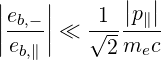
Because eb,- is the dominant polarization component and  ≪ 1, the second term in the sum
in (D.117) is largely dominant. We obtain
≪ 1, the second term in the sum
in (D.117) is largely dominant. We obtain
 | (D.118) |
For the O-mode, things are more complicated. However, if  ≪ 1, eb,∥ is much larger than
eb,-. The last term in (D.117) is dominant if
≪ 1, eb,∥ is much larger than
eb,-. The last term in (D.117) is dominant if
 | (D.119) |
which is satisfied for resonant electrons as long as the temperature is not too low. In that case, we have
 | (D.120) |
The vector Φb describes the relation between the energy flux and the electric field. In the cold plasma description, it is given by (4.287).
![*
ΦbP = Re [Nb - (Nb ⋅eb)eb]](NoticeDKE5363x.png) | (D.121) |
In general, both terms must be kept. However, where the density is low
 | (D.122) |
the ECW is mostly electromagnetic and mostly keeps its free-space characteristics. In that case,
| Nb | ≃ 1 | (D.123) |
 | ≪ 1 | (D.124) |
so that
 | (D.125) |
 ≪ 1 and ωpe ≪ ωb - or EM - approximations
The normalized bounce-averaged diffusion coefficient for the Fokker-Planck equation is given by (4.331)
| Db,nEC(0)(p,ξ 0) | =      ΨθbDb,n,0EC,θb
× ΨθbDb,n,0EC,θb
× | ||
H H H ![[ ]
1-∑
2
σ](NoticeDKE5375x.png) T δ T δ  2 2 | (D.126) |
with
| Db,n,0EC,θb | =     Pb,inc Pb,inc | (D.127) |
| N∥resθb | =    | (D.128) |
where we used the substitution n′→ n as in (D.111).
Within the small FLR,  ≪ 1 and ωpe ≪ ωb - or electromagnetic - approximations, we
have obtained the following expressions for the ECW properties (D.118), ( D.120),
(D.125)
≪ 1 and ωpe ≪ ωb - or electromagnetic - approximations, we
have obtained the following expressions for the ECW properties (D.118), ( D.120),
(D.125)
| Θkb,EC-Xn | ≃ e+iα  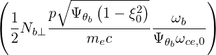 n-1 n-1 | (D.129) |
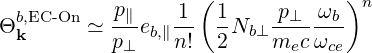
| Θkb,EC-On | ≃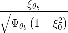 eb,∥ eb,∥  n n | (D.130) |
| ΦbEC | ≃ b b | (D.131) |
so that

In addition, within these approximations, the polarizations take the following limit expressions:
 | (D.132) (D.133) |
We consider the limit of a tokamak with circular flux-surfaces. In that case, we have the following identities
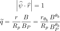 | (D.134) (D.135) |
| DbEC-Xn(0)(p,ξ 0) | =    ΨθbDb,n,0EC,θb ΨθbDb,n,0EC,θb
![-----1-----
4[(n- 1)!]2](NoticeDKE5399x.png) | ||
×  2 2    2 2 | |||
× H H H  ![[ ]
1 ∑
2-
σ](NoticeDKE5409x.png) T exp T exp![[ ( ) ]
- N ∥res - Nb ∥,0 2
------ΔN--2------
∥](NoticeDKE5410x.png) | (D.136) |
| DbEC-On(0)(p,ξ 0) | =    Db,n,0EC,θb Db,n,0EC,θb
![-1--
[n!]2](NoticeDKE5414x.png) | ||
×  2n 2n n n 2n 2n | |||
× H H H  ![[ ]
1 ∑
--
2 σ](NoticeDKE5421x.png) T exp T exp![[ ]
- (N ∥res - Nb ∥,0)2
----------2------
ΔN ∥](NoticeDKE5422x.png) | (D.137) |
with
| Db,n,0EC,θb | =    finc,bl+1∕2P
b,inc finc,bl+1∕2P
b,inc | (D.138) |
| N∥resθb | =    | (D.139) |
and where we assume a gaussian power spectrum as in (4.355).
In order to compare with ECCD operators found in the litterature, we redefine the EC constant factors such that
| DbEC-Xn(0)(p,ξ 0) | =   2 2  Db,0,newEC-Xn,θb Db,0,newEC-Xn,θb
  | ||
H H H ![[ ]
1-∑
2 σ](NoticeDKE5437x.png) T exp T exp![[ ( )2]
---N-∥res --Nb∥,0-
ΔN ∥2](NoticeDKE5438x.png) | (D.140) |
with
| Db,0,newEC-Xn,θb | =  ![1
----------2
4 [(n - 1)!]](NoticeDKE5440x.png)  2 2 D
b,n,0EC,θb D
b,n,0EC,θb
| (D.141) |
=     ![-----1-----
4 [(n - 1)!]2](NoticeDKE5447x.png)  2 2 f
inc,bl+1∕2P
b,inc f
inc,bl+1∕2P
b,inc | (D.142) |
and
| DbEC-On(0)(p,ξ 0) | =   2n 2n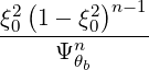 Db,0,newEC-On,θb Db,0,newEC-On,θb
 | ||
H H H ![[1 ∑ ]
--
2 σ](NoticeDKE5456x.png) T exp T exp![[- (N - N )2]
-----∥res--2-b∥,0--
ΔN ∥](NoticeDKE5457x.png) | (D.143) |
with
| Db,0,newEC-On,θb | =  ![--1-
[n!]2](NoticeDKE5459x.png)  2nD
b,n,0EC,θb 2nD
b,n,0EC,θb
| (D.144) |
=     ![-1-2
[n!]](NoticeDKE5465x.png)  2nf
inc,bl+1∕2P
b,inc 2nf
inc,bl+1∕2P
b,inc | (D.145) |
The two most common ECCD scenarios in experiments are the ones with the largest diffusion coefficient: X2 and O1. For these case, we find
| DbEC-X2(0)(p,ξ 0) | =   2 2 Db,0,newEC-X2,θb Db,0,newEC-X2,θb
 | ||
H H H ![[ ]
1 ∑
--
2 σ](NoticeDKE5473x.png) T exp T exp![[ ( ) ]
- N ∥res - Nb∥,0 2
----------2------
ΔN ∥](NoticeDKE5474x.png) | (D.146) |
with
 | (D.147) |
and
| DbEC-O1(0)(p,ξ 0) | =   2 2 Db,0,newEC-O1,θb Db,0,newEC-O1,θb
 | ||
H H H ![[ ∑ ]
1-
2 σ](NoticeDKE5482x.png) T exp T exp![[ ( )2]
---N-∥res --Nb∥,0-
ΔN ∥2](NoticeDKE5483x.png) | (D.148) |
with
 | (D.149) |