Bounce integrals

5.1 Bounce integrals

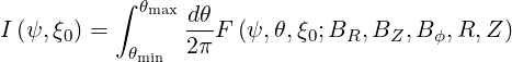
The numerical calculation of bounce coefficients requires an integration over θ which can be expressed symbolically as

∫ θmaxdθ I (ψ, ξ0) = ---F (ψ,θ,ξ0;BR, BZ,B ϕ,R,Z ) θmin 2π

(5.1)

where B_R,B_Z,B_ϕ,R,Z are functions of (ψ, θ) . They are given on a uniform grid of N_θ points in θ

θj =--2πj--,j = 0,1,⋅⋅⋅,N θ - 1 N θ - 1

(5.2)

Domain of Integration It is very important to account for the entire bounce path of the particle, including in particular the tip of banana orbits near θ_{T min} and θ_{T max}. The contribution of these banana tips is often larger than the dθ = 2π∕(N_θ - 1) accuracy level, because F (θ ) can become very large near the turning points. This is true for example in the calculation of λ, since F (θ) ~ 1∕ξ and ξ → 0 at the turning points. It is therefore crucial to perform the integration up to θ_{T min} and θ_{T max}. However, these boundaries are defined by (2.28) and (2.29)

B0 (ψ ) B (ψ,θT ) = Bb (ψ,ξ0) =----2- 1- ξ0

(5.3)

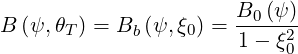
which in general do not coincide with a grid points. In order to calculate θ_T, we impose that the values of the data B_R,B_Z,B_ϕ,R,Z in θ_T be obtained by linear interpolation, while the value of B (ψ,θT ) is obtained from (2.30).

We consider the magnetic field B_b (ψ,ξ )
0 at the turning point θ_{T min} to be located between the two (consecutive) values B₁ (ψ, θ1) and B₂ (ψ,θ2) on the (ψ,θ) grid. These values are determined from the three components issued by the equilibrium code simply by

∘ --------------------------------- B (ψ,θ ) = B2 (ψ,θ )+ B2 (ψ, θ) + B2 (ψ,θ ) (5.4) 1 1 ∘ -R-----1-----Z-----1----ϕ-----1-- B (ψ,θ ) = B2 (ψ,θ )+ B2 (ψ, θ) + B2 (ψ,θ ) (5.5) 2 2 R 2 Z 2 ϕ 2

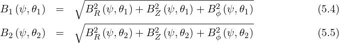
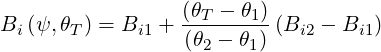
We choose to define the values of B_R, B_Z and B_ϕ at the location θ_T by linear interpolation:

B (ψ,θ ) = B + (θT---θ1)(B - B ) i T i1 (θ2 - θ1) i2 i1

(5.6)

where i = R,Z,ϕ. Then, the location θ_T of the turning point can be calculated by requiring that the relation

∘ ---------------------------------- 2 2 2 Bb(ψ, ξ0) = B (ψ,θT) = B R(ψ,θT )+ B Z (ψ,θT )+ B ϕ(ψ,θT)

(5.7)

be satisfied. This implies

B2 (ψ, θ )+ B2 (ψ, θ )+ B2 (ψ,θ ) = B2 (ψ,ξ ) R T Z T ϕ T b 0

(5.8)

and then

∑ [ (θT - θ1) ]2 Bi1 + ---------(Bi2 - Bi1) - B2b (ψ, ξ0) = 0 i=R,Z,ϕ (θ2 - θ1)

(5.9)

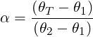
Defining

(θT - θ1) α = -(θ----θ-) 2 1

(5.10)

we find

⌊ ⌋ ⌊ ⌋ ⌈ ∑ (B - B )2⌉ α2 + 2⌈ ∑ B (B - B )⌉α + ∑ B2 - B2 (ψ,ξ ) = 0 i2 i1 i1 i2 i1 i1 b 0 i=R,Z,ϕ i=R,Z,ϕ i=R,Z,ϕ

(5.11)

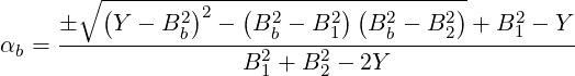
which solves as

∘ -∑--------------------[∑-------------][∑----------]- ∑ ± [ iBi1(Bi2 - Bi1)]2 - i(Bi2 - Bi1)2 iB2i1 - B2b - iBi1(Bi2 - Bi1) α = ------------------------------∑-------------------------------------------- i(Bi2 - Bi1)2

(5.12)

We have

┌ ------------------------------------------------------------- │ [ ]2 [ ][ ] │∘ ∑ B (B - B ) - ∑ (B - B )2 ∑ B2 - B2 (ψ, ξ) i1 i2 i1 i2 i1 i1 b 0 ∘ ---i---------------------i-----------------i----------- (BR1BR2 + BZ1BZ2 + Bϕ1B ϕ2)2 - B21B22 = + [B2 + B2 - 2(BR2BR1 + BZ2BZ1 + B ϕ2Bϕ1)]B2 (ψ,ξ0) ∘ -----2-----1-------------------- b = (Y - B2 )2 - (B2 - B2 )(B2 - B2 ) (5.13) b b 1 b 2

with

Y = BR1BR2 + BZ1BZ2 + B ϕ1Bϕ2

(5.14)

so that

∘ (-------)2--(--------)(--------) ±----Y---B2b-----B2b --B21-B2b --B22-+-B21---Y αb = B2 + B2 - 2Y 1 2

(5.15)

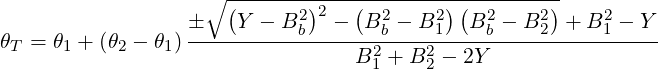
and finally

∘ -------------------------------- ( 2)2 ( 2 2) ( 2 2) 2 θ = θ + (θ - θ ) ±---Y---Bb------Bb---B1---Bb---B2--+-B-1 --Y- T 1 2 1 B21 + B22 - 2Y

(5.16)

We must choose (numerically) the solution that gives 0 ≤ α_b ≤ 1. Note that if the magnetic fields in points 1 and 2 are equal, we have Y = B₁² = B₂² = B_b².

Numerical Integration Once the two turning points have been added to the θ grid, now noted ^
θ _j, j = 0,1,2, ⋅⋅⋅ N_θ + 1, we define the half grid

( ) ^θ + ^θ θ- = ---k+1----k--,k = 0,1,2,⋅⋅⋅N k 2 θ

(5.17)

and calculate the discrete function

( -- ) Fk = F ψ,θk,ξ0;BRk, BZk, Bϕk,Rk, Zk

(5.18)

where B_Rk,B_Zk,B_ϕk,R_k,Z_k have been calculated on the grid θ_k by linear interpolation, and the step dθ_k, defined by

--- ^ ^ dθk = θk+1 - θk,k = 0,1,2,⋅⋅⋅N θ

(5.19)

so that the integral becomes

N∑θ --- I (ψ,ξ0) = 1- dθkFk 2π k=0

(5.20)

[next] [prev] [prev-tail] [front] [up]