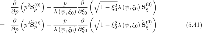
The starting point of the numerical calculations for the Fokker-Planck equation is the following expression
 is the bounce-averaged avalanche source term that comes into play in runaway
regime. In order to avoid numerical singularities at p = 0, it is convenient to multiply all the
terms by the partial Jacobian
is the bounce-averaged avalanche source term that comes into play in runaway
regime. In order to avoid numerical singularities at p = 0, it is convenient to multiply all the
terms by the partial Jacobian
 | (5.34) |
which leads to the equivalent form
![[ ]
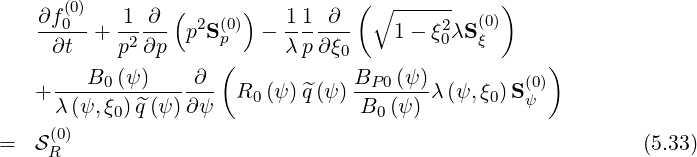
∂ -^q(ψ)-p2f(0) ∕∂t
B0 (ψ) 0
^q(ψ) ∂ ( )
+ --------- p2S (0p)
B0 (ψ)∂p (∘ ------ )
- -^q(ψ)----p-----∂-- 1 - ξ2λ(ψ, ξ) S(0)
B0 (ψ)λ (ψ,ξ0)∂ξ0 0 0 ξ
p2 ∂ ( B (ψ) )
+ ----------- R0(ψ )^q(ψ) -P-0---λ (ψ,ξ0)S(ψ0)
λ (ψ, ξ0)∂ψ B0 (ψ)
-^q(ψ-) 2 (0)
= B0 (ψ)p RSR (5.35)](NoticeDKE2706x.png)
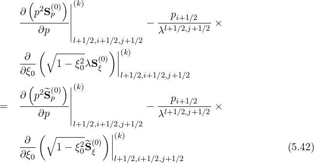
Using the grid definition defined in Sec.5.2 and applying the backward time discretization, which corresponds to the fully implicit time differencing as discussed in Sec. 6.1.1, the discrete form of the Fokker-planck equation may be expressed as
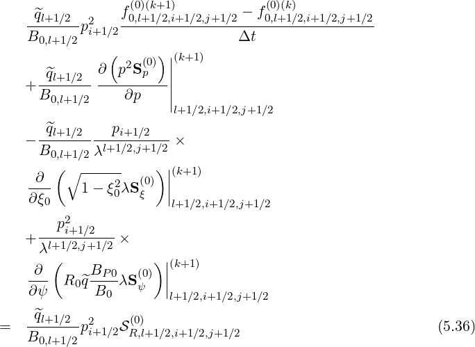
 l+1∕2 =
 , B0,l+1∕2 = B0
 and λl+1∕2,j+1∕2 = λ
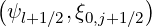 . In a
compact form
. In a
compact form 
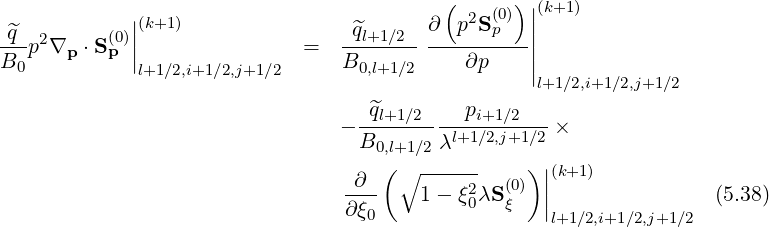
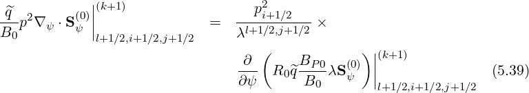
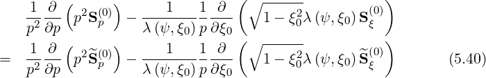
Since the first order drift kinetic equation may be also expressed in a conservative form as for the Fokker-Planck one as shwon in Sec. 3.5.5, a similar formalism may be kept. In that case,

 which is to be
determined, knowing
which is to be
determined, knowing  p
p and
and  ξ
ξ from the spatial derivative of f0
 given by the
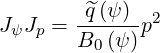
zero order Fokker-Planck equation. Multiplying also both sides by the partial Jacobian JψJp
defined in Sec. 3.5.1, one obtains
given by the
zero order Fokker-Planck equation. Multiplying also both sides by the partial Jacobian JψJp
defined in Sec. 3.5.1, one obtains