Boltzman equation; Gyro- and Wave-averaging

3.1 Boltzman equation; Gyro- and Wave-averaging

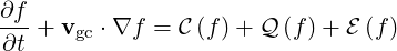
In the kinetic description, electrons are described by a distribution function f (r,p,t) , which gives the density in phase space of particles with a momentum p at a position r and at time t. The particle conservation equation in phase space is the Boltzmann equation

| ∂f ∂f | -∂t + v⋅ ∇rf + qe[E (r,t)+ v × B (r,t)]⋅∇pf = ∂t-|| C

(3.1)

where

∂f|| --|| ≡ C (f) ∂t C

(3.2)

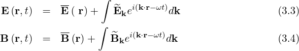
is the collision operator. The fields E (r,t) and B (r,t) are assumed to consist of time-independent macroscopic fields E (r) and B (r) and fields associated with plane waves.

∫ E (r,t) = E-( r)+ ^E ei(k⋅r-ωt)dk (3.3) ∫ k -- ^ i(k⋅r-ωt) B (r,t) = B (r)+ Bke dk (3.4)

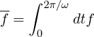
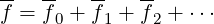
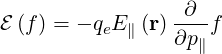
Because we are interested in solving the kinetic equation on the bounce and collisional time scales, we need to average over the faster time scales, which are the gyromotion and the wave oscillation.

Performing a time-averaging ∫ ₀^2π∕ωdt of the equation (3.1) removes the fast wave time scale from the equation, to give

∂f- -- [-- -- ] -- ---+ v ⋅∇rf + qe E (r)+ v × B (r) ⋅∇p f ∂t-| ∫ 2π∕ω ( [ ] ) = ∂f-|| - dt∑ q ^E + v × ^B ⋅∇ f (3.5) ∂t |C 0 e k k p k

where

-- ∫ 2π∕ω f = dtf 0

(3.6)

is the wave-period averaged distribution function. The time derivative in the first term of (3.5) implicitely refers to times longer than the wave period ω.

Under the assumption of a strong magnetic field, such that the gyrofrequency Ω_e

-- qeB Ωe = ---- γme

(3.7)

is much larger than both the collisional frequency and the bounce frequency, we can expand the distribution function

-- -- -- -- f = f0 + f1 + f2 + ⋅⋅⋅

(3.8)

with a small parameter

ωb νc δ ~ --- ~ --- Ωe Ωe

(3.9)

The zero order equation becomes

-- -- qev × B (r)⋅∇p f0 = 0

(3.10)

We have, in the ( )
p∥,p⊥,φ space defined in Appendix A,

-----p------ v = γ(p∥,p⊥) me

(3.11)

with the momentum being given by relation (A.214)

^ ^ p = p∥∥+ p⊥ ⊥

(3.12)

and the gradient by expression (A.239)

-- -- -- -- ∂f ∂f 1 ∂f ∇p f = ---^∥ + ----^⊥ + ------^φ ∂p∥ ∂p⊥ p⊥ ∂φ

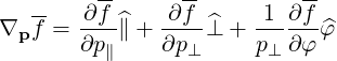(3.13)

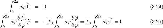
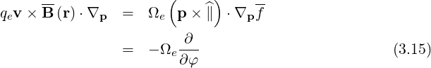
In this system, by definition,

-- -- B (r) = B (r)^∥

(3.14)

so that the gyromotion operator becomes

-- ( ^ ) -- qev × B (r)⋅∇p = Ωe p× ∥ ⋅∇p f ∂ = - Ωe--- (3.15) ∂φ

The equation (3.10) becomes consequently

-- ∂f0 ----= 0 ∂φ

(3.16)

and therefore f₀ is independent of φ. The first order equation is

∂f- -- -- -- -- ---0+ v ⋅∇rf0 + qeE (r)⋅∇p f0 + qev × B (r)⋅∇p f1 ∂t-| ∫ 2π∕ω ( [ ] ) = ∂-f0|| - dt∑ q ^E + v × ^B ⋅∇ f (3.17) ∂t |C 0 e k k p k

The last term in the equation (3.17) has been calculated by Lerche for a uniform plasma, in the form of a quasilinear operator (-)
f . We can rewrite

-- --|| C (f0) = ∂-f0| ∂t |C

(3.18)

(--) ∫ 2π∕ω ∑ ( [ ] ) Q f 0 = - dt qe ^Ek + v × ^Bk ⋅∇pf 0 k

(3.19)

Performing the gyro-averaging ∫ ₀^2πdφ on the kinetic equation (3.17), we find, using (3.16), that

∫ 2π ∂f^0 ∂ ^f0 d φ-∂t-= -∂t- 0

(3.20)

and

∫ 2π -- ∫ 2π -- -- dφv ⋅∇rf 0 = (d φv) ⋅∇rf0= vgc ⋅∇r f0 0 0

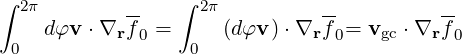(3.21)

where v_gc is the electron velocity along the guiding center.

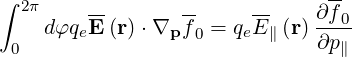
Concerning the electric field, we decompose the gradient in momentum space using (3.13)

-- -- -- ∫ 2π -- -- -- ∫ 2π [ ∂f0 ∂f 0 1 ∂f 0 ] dφqeE (r)⋅∇p f0 = qeE (r)⋅ dφ ∂p-^∥ + ∂p--^⊥ + p---∂φ-^φ (3.22) 0 -- 0 ∥ ⊥ ⊥ ∂-f0-- ^ = qe∂p ∥E (r)⋅∥ -- ∫ 2π +qe ∂f-0E-(r)⋅ dφ ^⊥ ∂p⊥ 0 -- qe -- ∫ 2π ∂f0 + ---E (r)⋅ dφ ----^φ (3.23) p⊥ 0 ∂ φ

and, using

∫ 2π dφ⊥^ = 0 (3.24) ∫ 2π 0 -- ∫ 2π ∫ 2π dφ ∂f-0^φ = - f- dφ ∂^φ-= f- dφ⊥^ = 0 (3.25) 0 ∂ φ 0 0 ∂φ 0 0

we obtain

∫ -- 2π -- -- -- ∂f0- 0 dφqeE (r)⋅∇p f0 = qeE∥ (r) ∂p∥

(3.26)

The gyromotion term is averaged to zero

∫ 2π -- -- ∫ 2π ∂f- dφqev × B (r)⋅∇p f 1 = - Ωe dφ --1-= 0 0 0 ∂φ

(3.27)

so that we get finally

( ) ( ) ∂-^f0+ v ⋅∇ f^ + q E--∂--(r) ^f = C ^f + Q ^f ∂t gc r 0 e ∥∂p ∥ 0 0 0

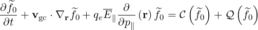(3.28)

This equation is called electron drift-kinetic equation. Renaming the guiding-center distribution function f₀ = f ( )
r,p∥,p⊥,t , E (r) = E (r) and B (r) = B (r) , we get

∂f -∂t + vgc ⋅∇f = C(f) + Q (f)+ E (f)

(3.29)

where we define an electric field operator

∂ E (f ) = - qeE∥(r)--f ∂p ∥

(3.30)

Implicitely, the time scale here considered is so that t ≫ (2π∕ω,2π ∕Ωe) .

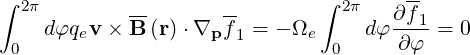
[next] [prev] [prev-tail] [front] [up]