B.4 Wave scattering by fluctuations
Low frequency fluctuations of the electron density or the magnetic field can strongly affect the
propagation of rf waves in a magnetized plasma. This effect has been extensively investigated
for the Lower Hybrid wave by solving a wave kinetic equation in the weak turbulence
approximation. [14, 15]. In this approach, the flow of rf energy is described by a usual
ray-tracing between random scattering events where the initial wave vector k can be modified
both in amplitude and direction with the constraint to remain solution of the local
dispersion relation. This physical mechanism is a good candidate for explaining a possible
strong upshift of the power spectrum as the Lower Hybrid wave propagates in the
plasma, even if the toroidal mode coupling for bridging the spectral gap is very weak.
Though primarily dedicated to the Lower Hybrid wave, the concept of wave scattering
by low frequency density or magnetic field fluctuations can be easily extended to
other types of rf waves provided that  ∥ ≪ k∥ and
  ≪ ω, where k∥ = k ⋅ b and
 ∥ =
∥ =  ⋅ b are the projections of the rf and fluctuation wave vectors respectively along
the direction of the local magnetic field b = B∕
⋅ b are the projections of the rf and fluctuation wave vectors respectively along
the direction of the local magnetic field b = B∕ , while ω and
  are the rf and
fluctuation frequencies respectively. Consequently, the scattering process becomes
a two dimensional problem in the plane perpendicular to the local magnetic field
direction, a reasonable assumption regarding the large difference between the long wave
length of the low frequency fluctuations and the short length of the rf waves along
b.
are the rf and
fluctuation frequencies respectively. Consequently, the scattering process becomes
a two dimensional problem in the plane perpendicular to the local magnetic field
direction, a reasonable assumption regarding the large difference between the long wave
length of the low frequency fluctuations and the short length of the rf waves along
b.
Calculations are organized in three steps. In the first section, the components of the
scattered rf wave vector are calculated, according to the curvilinear coordinate system
chosen for describing the magnetic equilibrium in C3PO. The wave kinetic equation
corresponding to the wave-wave interaction is then derived from first principles in the
second section. Finally, in the third section, the wave kinetic equation is solved using a
Monte-Carlo method and the procedure for the numerical implementation in the code is
explicited.
Before entering into the details of the calculations, it is possible to estimate the impact of a
simple transfer from the toroidal mode number n to the poloidal one m at fixed k∥0 on the ray
properties, by changing the initial conditions. The benchmark case presented in Sec.E.1 is
considered using Nϕ0 = -1.8. From a scan of m∈ with steps Δm = 50, it is
possible to show that a variation of m and n strongly affect the ray propagation, even if k∥0
remains unchanged.
with steps Δm = 50, it is
possible to show that a variation of m and n strongly affect the ray propagation, even if k∥0
remains unchanged.
B.4.1 Calculation of the scattered wave vector
When the rf wave vector k is scattered by low density fluctuations, it may change both in
module and direction, with the conditions
 | (135) |
where k′ is the scattered wave vector. Its perpendicular component k
⊥′ =  , where
k⊥′ = k′× b, is determined by solving the local dispersion relation (??) at fixed k
∥, and its
direction results from a rotation
, where
k⊥′ = k′× b, is determined by solving the local dispersion relation (??) at fixed k
∥, and its
direction results from a rotation  β of an angle β around the magnetic field direction b so
that
β of an angle β around the magnetic field direction b so
that
 | (136) |
For unlike transitions, the scattered wave moves to a different branch of propagation
and k⊥′≠k
⊥, otherwise k⊥′ = k
⊥ for like transitions. From the relations (??), (??)
and (??), all the components  of k′ can be deduced from those of
k.
of k′ can be deduced from those of
k.
The wave scattering may be therefore described as a two steps process, and the mode
conversion  and the rotation β.
B.4.2 Derivation of the wave kinetic equation
B.4.3 Solution of the wave kinetic equation
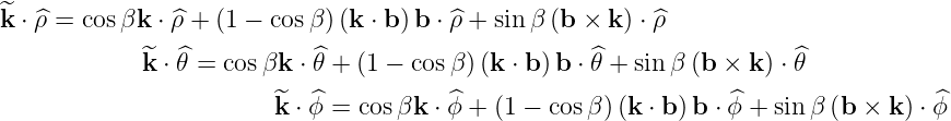
Using the Rodrigues general formula for the rotation β of a vector k,
 | (137) |
it turns out that each components of  is given by the relations
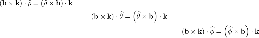
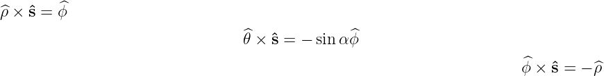
Using the vectorial relations
and
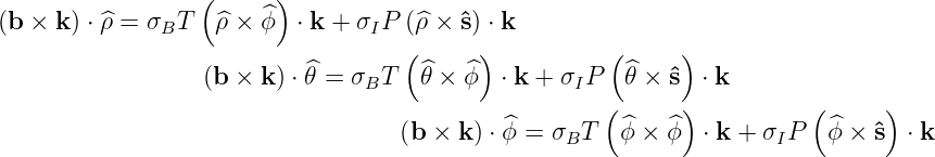
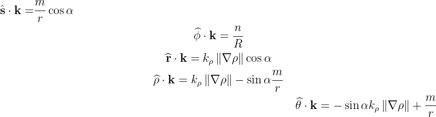
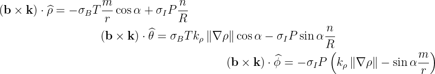
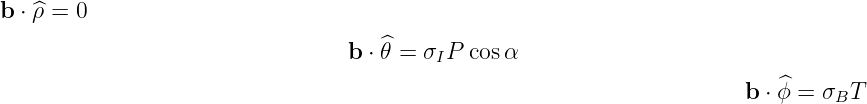
the expression on the magnetic field b = σBT + σIPŝ according to the relation (??), recalling
that T = BT ∕B and P = BP ∕B, one obtains which simplifies to since
and
using
the relations
+ σIPŝ according to the relation (??), recalling
that T = BT ∕B and P = BP ∕B, one obtains which simplifies to since
and
using
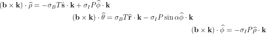
the relations  = sin α
 + cos α
 and
and  =
=  ×
× . Using (??), and
Finally, since
one
obtains or
 |
(138)
|
where k ⋅ b = k∥ and the scattered wave vector is
 | (139) |
If β = 0, it is straightforward to demonstrate that  = k. In addition, the relation
 ⋅ b = k ⋅ b or
 | (140) |
is also well satisfied whatever β, as expected from the initial assumption on the invariance of k∥
with the rotation of angle β, which is intrinsically considered in the Rodrigues formula
(??).
In the cold limit approximation, the plasma has bi-refringent optical properties which means
that for a given k∥, the dispersion relation cannot have more than two different roots in
k⊥.
From the definitions k⊥ = k × b and k⊥′ = k′× b, the relation k
⊥⋅ k⊥′ = k
⊥k⊥′ cos β
becomes

and
 | (141) |
For like mode scattering, k⊥′ = k
⊥ and
 | (142) |
a relation which can be well verified by replacing  from (138) into (??).
Therefore, for like mode scattering,
from (138) into (??).
Therefore, for like mode scattering,  have just to be deduced from (138) knowing
 .
.
For unlike mode scattering, k⊥′≠k
⊥,
Therefore, The coordinates of k′ are therefore determined by relations (??) and (??) and
(??),
 | (143) |
By definition, the variation of the poloidal mode number m is made possible by the breaking
of the toroidal symmetry resulting from the fluctuations, so that the toroidal mode number n is
no more conserved in the scattering process.