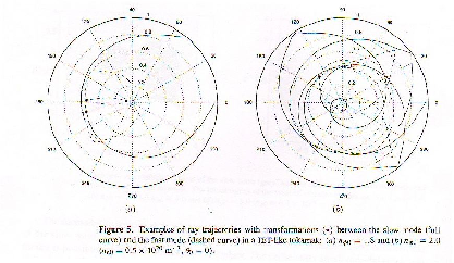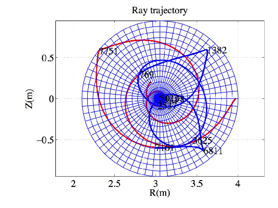
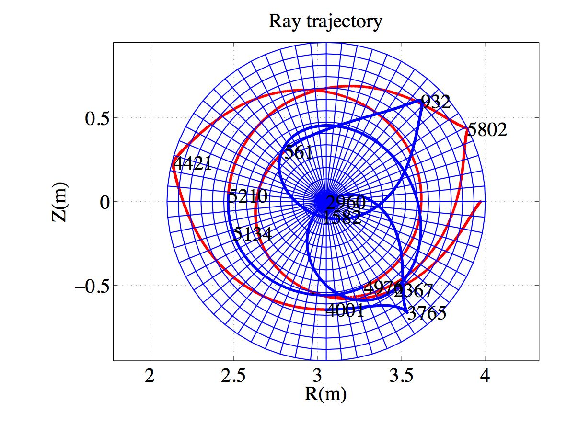
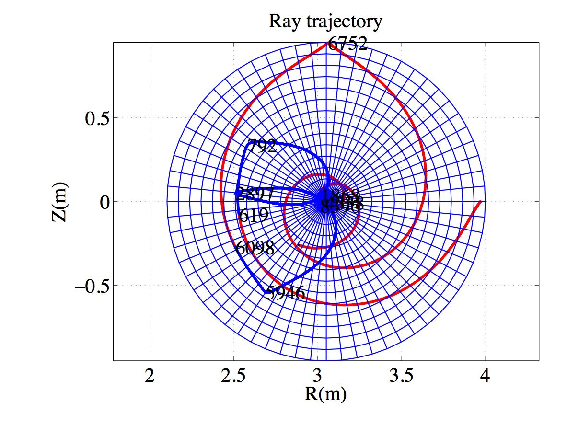
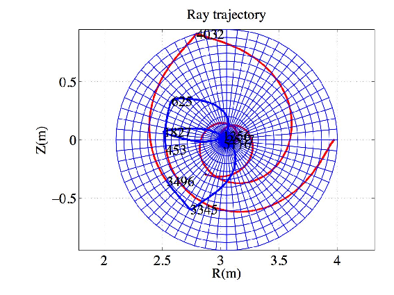
Figure 1: Poloidal projection of the ray trajectory. The red curve corresponds to the
slow mode and the blue curve corresponds to the fast mode. Numeric (upper plot) and
analytic (lower plot) magnetic equilibrium. Nϕ0 = -2.0
A JET-like equilibrium was used in Ref.[16] where results from a ray-tracing code using the cold plasma model is presented. A circular concentric toroidal plasma is considered such that
 | (151) |
with the following equilibrium parameters
 | (152) |
and the following profiles
 | (153) |
with
 | (154) |
The total current is then
 | (155) |
such that
 | (156) |
The magnetic field profile is
 | (157) |
Ampere’s law gives in the small aspect ratio limit (consistent with concentric flux surfaces)
 | (158) |
we get
 | (159) |
with
 | (160) |
The poloidal flux coordinate ψ = Rp ∫ 0rB P dr is then
 | (161) |
In the case α = 1 it gives
 | (162) |
Defining ρ = sin θ

yields
and finally for α = 1 we gather

Note that the q profile is approximately (to order ϵ)
 | (164) |
which gives
 | (165) |
and for α = 1
 | (166) |
where
 | (167) |
Note that q = qmax∕(1 + α) and dq∕dρ
 = 0.
= 0.
The ray is launched in the slow mode from the position
 | (168) |
with the spectral properties
 | (169) |
From (??) the initial n can be determined
 | (170) |
and then the parallel index of refraction is
 | (171) |
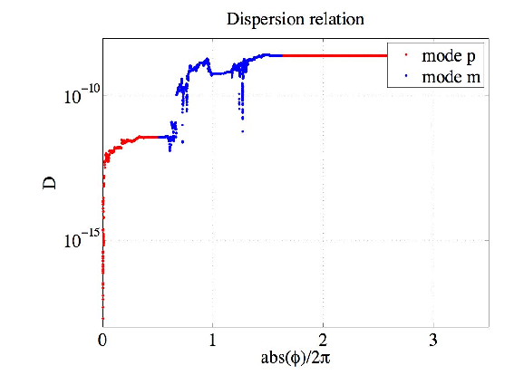
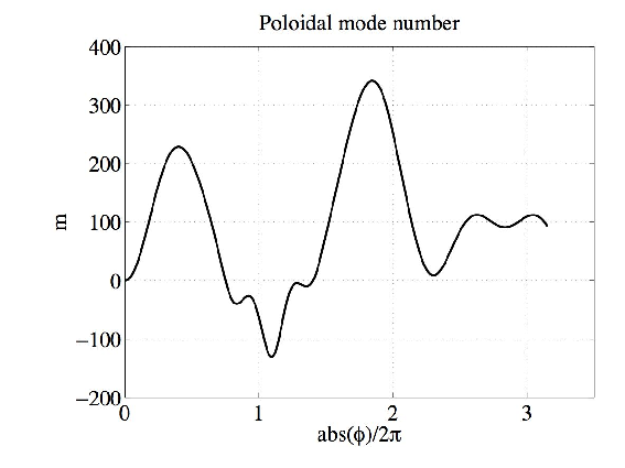
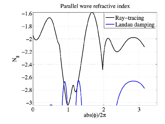
The results are plotted in figures 1-6. The wave is mode-converted between the slow to the fast mode several times. The results agree remarkably well with those from Ref.[16]. A small difference in the ray path between the analytical and the interpolated magnetic equilibria is observed in the case Nϕ0 = -1.8. The deviation is certainly due to the ray passing near the center of the plasma where the numerical interpolation is intrinsically less accurate.
The magnetic equilibrium is defined on a numerical grid of size 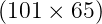 along the radial
and poloidal direction respectively. It is vectorized using a Fourier series expansion
with 32 harmonics and the Matlab built-in cubic spline interpolation for the Fourier
coefficients. The vectorization procedure takes typically 8.3 seconds on computer equipped
with a 64 bits biprocessor AMD opteron clocked at 2.4 GHz, with 4 GBytes of RAM
memory.
along the radial
and poloidal direction respectively. It is vectorized using a Fourier series expansion
with 32 harmonics and the Matlab built-in cubic spline interpolation for the Fourier
coefficients. The vectorization procedure takes typically 8.3 seconds on computer equipped
with a 64 bits biprocessor AMD opteron clocked at 2.4 GHz, with 4 GBytes of RAM
memory.
Ray calculation parameters for the example presented here are typical of tokamak current drive simulation. Ray parameters are stored in the memory each time the radial increment Δρ is larger than 10-4. Δρ may be adapted depending upon the problem. In the 6th order Runge-Kutta procedure, the generalized incremental step h is adjusted so that the norm6 of the variation along the six directions of extrapolation never exceeds the tolerance level which is set to 10-12. The tolerance level is arbitrarily chosen so that the ray trajectory as well as all wave parameters are independent of its value. Below 10-12, the gain on the ray accuracy is marginal while the computer time increases.
The initial time increment is set to h0 = 10-4 in normalized units, and the calculation ends when tend = 10000, with a maximum of 60000 values stored in the memory. Since the time step h evolves along the ray trajectory depending upon the ray curvature, the effective number of steps is typically much less that tend∕h0. For the current example tend is reached after 5499 steps.
Using the numerical equilibrium, the ray trajectory is calculated in 35.15 seconds, while it takes only 1.21 seconds with the analytic equilibrium. Although the numerical equilibrium is more time consuming by at least an order of magnitude, typical calculation times remain at an acceptable low level for realistic time-dependent tokamak simulations, which require several hundred ray trajectories calculations.