D.1 Cold Plasma Model

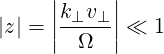
In this section, we use the cold plasma model to calculate the wave properties. This approximation is valid only if the following conditions are satisfied:

• The wave must exist in the cold plasma model, which is not the case of electrons Bernstein waves (EBW). The description of EBW requires a hot plasma model.
• The wave remains far from resonances, where k_⊥ → ∞. Near resonances, mode conversion to electrostatic waves (IBW, EBW) occur, which are not described by cold plasma wave theory. LHCD and ECCD usually take place far enough from the LH and UH resonances, respectively, so that the cold plasma description is valid.
• Hot plasma effects, such as the energy flow carried by the coherent motion of particles Φ_bT , must be negligible.
• FLR effects must be small, that is, we must have

  (D.1)

  This condition generally holds for LHW and ECW as long as the temperature is not too high (T ≤ 10 keV) and the resonance harmonic is low (n = 0,1,2).

In the first subsection, we discuss the modeling of RF k_∥ spectrum. In the second subsection, we use the cold plasma model to calculate wave properties. In the third and fourth subsections, we use further approximations to give analytical formulas for the properties of LHW and ECW. This leads to a simplified description of LHCD and ECCD and allows us to compare our models and results with other codes.

D.1.1 Wave Equation and Dispersion Tensor

We consider the two-fluids description of a non relativistic plasma in a constant magnetic field B₀ = B₀ . In a continuous homogeneous linear medium, a Fourier component E_b verifies the wave equation [?]

(D.2)

or equivalently

(D.3)

where N_b = ck_b∕ω_b is the wave refractive index and K is the dielectric tensor. This equation can be expressed in tensorial form as

(D.4)

where the dispersion tensor is

(D.5)

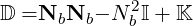
By evaluating the susceptibilities in the cold plasma limit, the following dielectric tensor is obtained [?] in the frame :

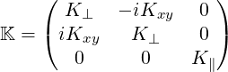(D.6)

whose elements in a plasma made of species s are given by

K⊥	= 1 -∑ s
K∥	= 1 -∑ s
Kxy	= -∑ s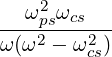	(D.7)

where

(D.8)

is the plasma frequency and

(D.9)

the cyclotron frequency for the species s.

D.1.2 Dispersion Relation

In order to have a non-trivial solution to the wave equation, the dispersion relation must therefore be satisfied:

(D.10)

The axis is chosen such that

(D.11)

Taking the parallel component N_b∥ as given, (D.10) lead to the following equation for N_b⊥

(D.12)

with

A	= K⊥	(D.13)
B	= + Kxy2	(D.14)
C	= K∥	(D.15)

or equivalently

A	= K⊥	(D.16)
B	= Nb∥2 -	(D.17)
C	= Kb∥	(D.18)

with

We find the expression for N_b⊥ as a function of N_b∥ and ω:

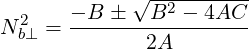(D.21)

We see immediately that the resonances occur for A = 0, that is,

(D.22)

and that cut-offs occur for C = 0, that is,

(D.23)

(D.24)

or

(D.25)

D.1.3 Polarization components

Once N_b⊥ has been evaluated, the components of the polarization of the electric field are simply given as the eigenvector of the wave equation (D.4)

(D.26)

D.1.4 Power flow

The relation between power flux and electric field was described using the vector Φ_b defined in (4.284)

(D.27)

with (4.287)

(D.28)

and (4.286)

(D.29)

In the cold plasma model, the dielectric tensor K is independent of N_b and the contribution Φ_bT , from the coherent motion of particles, vanishes.

(D.30)

It is usually a very good approximation to neglect this kinetic power flux, even for quasi-electrostatic waves like Lower-Hybrid waves (See D.2.7).

D.1.5 Conclusion

The cold plasma model gives expressions (D.21), (D.26) and (D.28) for the calculation of N_⊥, e_b and Φ_b respectively. These formulas can be generally used for the calculation of the diffusion coefficient in LHCD and ECCD.